This chapter focuses on structuring the data needed to
represent the objects and their characteristics significant for the municipality
governance. For this purpose, first the requirements derived in Chapter
3 and Chapter 4 are summarised. Second,
a generalised definition of objects is proposed, which provides a framework
for structuring the information collected per object, regardless of the
type of object. The data per object are distinguished on the basis of their
thematic and geometric origin. Under the assumption that the objects with
spatial extent are the more sophisticated for organisation, further elaboration
is provided only in the geometric domain. Three spatial topological models
are assessed for their suitability to 1) represent spatial objects and
spatial relations, and 2) ensure sufficient data for correct visualisation
in a short period of time. Motivated by the advantages and disadvantages,
a new spatial model is formulated in Section
5.5.
5.5.1 Objects: spatial and non-spatial5.3 Spatial models
5.2.2 Object components in the geometric domain5.2.2.1 Geometric appearance (GA)5.2.3 Composite objects
5.2.2.2 Geometric relationships (GR)
5.2.2.3 Geometric behaviour (GB)
5.3.1 3D FDS5.4 Arcs in spatial models
5.3.2 TEN
5.3.3 The cell tuple model
5.5.1 Definition of constructive objects5.6 SSM for urban modelling
5.5.2 Definition of geometric objects
The requirements outlined in the previous chapters refer to different aspects of a 3D GIS, i.e. modelling, analysis, visualisation and Web access. In accordance with the objectives of the research, i.e. an integrated conceptual model, the requirements have to be considered in their completeness. In other words, the organisation of data in the database (see Figure 4-7) must be appropriate for both 3D GIS analysis (thematic and spatial) and composition of documents (HTML and VRML). Recalling discussions from the previous chapters, we can summarise the requirements of the data and their structuring as follows:
The categorisation of real objects given in Chapter 3 as well as the approach for visualisation presented in Chapter 4 make claim for an extended object definition, capable of describing various characteristics of real objects.
5.5.1 Objects: spatial and non-spatial
The object definitions in geo-sciences (see Chapter 2) focus on spatial objects, with their geometric, radiometric properties, semantics, spatial relationships and time. As shown, our study requires broader understanding dealing with spatial and non-spatial objects. Therefore, we will start with general concepts applied in business processes, and will later make specifications for a spatial object. Among the common object-oriented approaches to identifying objects, we have chosen the one proposed by Coad because of the common notations for objects, responsibilities and scenario. The initial statement in Coad's definition, "the object can be anything: feature, action, process, which is of interest for the user", can be successfully applied to the variety of real objects of interest already identified. The object responsibilities and time-related component (scenario) can be utilised to complete a broad characterisation of any real object. Chapter 3 has used the basic principles of this OO approach to clarify objects of interest. This chapter applies the same principles to derive an extended definition of an object capable of describing spatial and non-spatial objects (see also Zlatanova and Gruber 1998).
An object O can be represented by two components OR (object responsibilities) and S (scenario): O (OR, S). The brackets here are notations for the expression consist of, i.e. the notation O (OR, S) has to be read an object consists of object responsibilities and scenario. Thus, considering the groups of real objects introduced in Chapter 3, we can distribute the information maintained in current information systems according to the meaning of object responsibilities and scenario (see Table 5-1).
Table 5-1 Object responsibilities and scenario of real objects
| Groups of
real objects |
What the object knows
about itself |
Who the object knows | What the object does | Scenario |
| Juristic | Attributes | Interrelations | Functions, Operations | Archive |
| Topographic | Shape and/or size,
location, attributes |
Spatial relationships | Functions, Operations | Archive |
| Fictional | Shape and/or size,
location, attributes |
Spatial relationships | Functions, Operations | Archive |
| Abstract | Attributes | Interrelations | Functions, Operations | Archive |
Coad's three questions refer to characteristics of objects, which here will be called attributes, relationships and behaviours. Attributes (A) comprise the characteristics, which identify the object on the basis of personal properties. Relationships (R) represent interactions (mostly static) of the object with other objects. Behaviours (B) refer to the dynamics (functions) of objects or dynamic interaction with other objects. Scenario represents the dynamics of objects with respect to the absolute time (days, months, years, etc.). Thus we write the three components of OR as:
OR (A,R,B)
The substitution of the OR components in the notations for an object O will give us the full set of components describing an object, i.e. attributes, relationships, behaviour and scenario:
O (A,R,B,S)
The preliminary, still generalised, notion of an object provides the first classification of the information per object. For example, the existing records about a person, a building, a district and a document can be mapped into the four components as follows:
Table
5-2: An example for a classification of the data per object
| Object | Components | Existing information | Extended information |
| Person | Attributes | PIN, name, address, marital status | |
| Relationships | Living house, agricultural land | ||
| Behaviour | CheckIn, CheckOut
Select, edit, delete, add data |
Lessons in music,
Web page |
|
| Scenario | Thee changes of the address | ||
| Building | Attributes | ID, hotel, made of bricks,
Address, size, shape, position |
|
| Relationships | Attached to the building of
the theater, part of chain of hotels, owner |
||
| Behaviour | Select, edit, delete, add data, show owner | Sightseeing from
the roof |
|
| Scenario | Building is reconstructed four
times,
last used as a hospital |
||
| District | Attributes | ID, district (centre), position, size, shape | |
| Relationships | Neighbour districts | ||
| Behaviour | Select, edit, delete, add | Provides
statistic information |
|
| Scenario | Boundary archives | ||
| Tax document | Attributes | ID, building tax, car tax, dog tax | |
| Relationships | PIN of the payer, address of the payer | ||
| Behaviour | TaxPaid
Select, Edit, delete, add |
||
| Scenario | Records of each year |
While acceptable for non-spatial objects, such classification of data is not sufficient to distinguish between semantics and geometry of spatial objects: 1) geometric and thematic characteristics are united behind attributes, e.g. the position of a building is together with the usage and 2) the spatial relationships are maintained together with thematic relationships. Therefore, we will further elaborate on components in the geometric (GD) and thematic (TD) domains:
O (GD, TD)
We introduce attributes, relationships, behaviour and scenario of spatial objects in the thematic and geometric domains:
GD (GA, GR, GB, GS)
TD (TA, TR, TB, TS)
where GA, GR, GB, GS - geometric appearance (will be discussed), geometric relationships, geometric behaviour, geometric scenario; TA, TR, TB, TS - thematic attributes, thematic relationships, thematic behaviour, thematic scenario
Thus the components of an object can be written as:
O ((GA, GR, GB, GS), (TA, TR, TB, TS))
While the thematic component is compulsory, the geometric one is optional per object. That is to say, if the geometric components do not exist, the object can be maintained only according to its thematic description. For example, documents or people commonly do not have geometric representations (see Chapter 4 for recent research). Similarly, not all the components within one domain are obligatory. For example, the geometric domain may be represented only by GA and GR or even only by GA (shape, size, position and colour of objects but not relationships). In general, the information that is maintained in current GISs corresponds to the information represented by the components GA, GR and TA, i.e. shape and position of spatial objects, spatial relationships and thematic attributes.
The components of objects with a clear differentiation between thematic and geometric information contribute to: 1) facilitation of the information structuring per object and 2) integration of spatial and non-spatial objects in one information system. The benefit for data organisation is threefold:
Inside the thematic and geometric components, spatial and non-spatial objects can be organised in an integrated database. The attributes, relations and behaviour of non-spatial objects will be limited to the thematic domain until the user introduces geometric description.
5.2.2 Object components in the geometric domain
The components in thematic domain (TD), are not further explored because of 1) their high dependence on particular user requirements, which were not investigated and 2) a variety of approaches and methods to structure semantic information (Norman, 1996). Consequently, we will preserve the detailed notation to the geometric domain, with an indication that, the thematic domain has to be considered as well, i.e.:
O((GA, GR, GB, GS), TD)
5.2.2.1 Geometric appearance (GA)
The component GA is referred to here as geometric appearance (not geometric attributes). The more complex meaning of the attributes in the geometric domain motivates the introduction of another term. The information about geometric characteristics (i.e. shape, position and size) and radiometric characteristics (i.e. reflectance) are intended to be represented by this component. As mentioned above, the 3D visualisation process needs these properties to create a 3D scene. Since they make feasible the appearance of the object in the scene, the term geometric appearance is used. The shape, size and position are implicit properties dependent on the manner of geometric description chosen, (e.g. vector representations, CSG, raster representations) and the abstraction principle applied. Variations can be quite significant. Colour, texture, material are determined by some physical properties (e.g. material used for covering roofs) of real objects and are not influenced by the geometric representation, i.e. they are explicit properties. For example, the roof of a building might be represented by red colour regardless of the geometric representation, e.g. a cone or a set of triangles. Therefore we introduce two new components: geometric description (GDsc) and geometric"attributes"(GAtt) as part of GA, i.e.
GA (GDsc,GAtt) => O (((GDsc, GAtt), GR, GB, GS), TD)
The component GDsc addresses shape, size and position and the GAtt is responsible for radiometric properties. The notation geometric attribute is introduced to indicate that this is a "personal" characteristic of the object (i.e. belongs to the group attributes) in the geometric domain.
Despite the three dimensions of every object, the modelling process still requires certain abstractions of real objects to be built. The historical human experience with maps and 3D CAD models has contributed to the establishment of four abstraction types of objects, i.e. points, lines, surfaces and solids. We will use the terms point, line, surface and body and will give them the common notation geometric objects (GO). The next distinction is between geometricobjects and constructive objects (CnsO). Geometricobjects are elementary nD objects (n = 0,1,2,3), which can be associated with thematic meaning, while constructive objects are used to compose geometric objects. They represent either shape and position or size and position of GO. For example, a house represented as body (GO) can be built of many cubes (CnsO) with different sizes and positions in the space. The same house can be built of many faces (CnsO) with different shapes and positions in the space. Although many spatial models use different CnsO, the geometric objects in 3D space are usually four, e.g. 3D FDS, TEN and the cell model (see Section 5.3).
The component geometric description is a function of constructive elements:
GDsc(GO[CnsO])
Then the geometric appearance is represented by two components geometric description and geometricattributes, where the geometric description is expressed by geometricobjects(GO), which are function of constructiveobjects(CnsO), i.e.
GA(GO(CnsO),GAtt)
The notation of an object is extended with the components containing more detailed information about GDsc:
O(((GO[CnsO],GAtt), GR, GB, GS), TD)
5.2.2.2 Geometric relationships (GR)
The second component in the geometric domain deals with geometric relationships (GR) or spatial relationships. The manner of representing spatial relationships is closely related to the method of description. If the representation in the GDsc component does not ensure the needed spatial relationships, some of them can be explicitly formulated, e.g. 3DFDS. GR and GDsc will be discussed in detail in Section 5.3 and Section 5.5.
5.2.2.3 Geometric behaviour (GB)
The third component, denoted geometric behaviour, focuses on permanent repeatable behaviours of real objects (e.g. opening of a door), which are preserved in the virtual world. The way to represent such dynamics is very similar to the interactions between the objects in the real world. For example, to open a door someone has to push the handle down, i.e. someone takes the initiative to open it. The same interaction has to be simulated in the virtual world, i.e. some event has to "take the initiative" to open the door. Since the door is open, a new view appears, i.e. there is a response event. Behaviour contains parameters needed to simulate such dynamics. Furthermore some actions might be allowed to some users and forbidden to others. Identically, in the real world not everyone has the right to destroy a particular house. In this respect, a control on the permitted operations on the object during navigation and editing has to be ensured. In addition to these considerations, the access, retrieval and display of data over Internet gains from organisation of behaviour at database level (see Chapter 4).
In the light of the VRML concepts and the CGI scripting, we can distinguish the following types of behaviour:
Operations on geometry (OG): This type refers to permitted operations on an object such as the generic operations (see Chapter 2): 1) deleting (OD) an existing object or some of its components, 2) updating (OU) some values of components of an existing object and 3) adding (OA) a new object or a new component of an object. Operations on geometry can be presented as a set of three components OG (OD, OU, OA). Further, we can specify which particular components are accessible to the user for modification. For example, we can forbid any changes in the components GDsc and allow changes only in GAtt.
Such behaviours, known as methods, are widely used in object-oriented programming to define different operations (see Chapter 2). The idea, here, is the organisation of behaviour at database level. Control of the operations on objects can be successfully used to protect the information on the GIS server. Since the tendency of our approach is to provide a broad range of users with access to the information, a strong security system against mistakes and unscrupulous actions has to be developed. Protection of data can be built up on two levels: server and database. The server level controls and restricts user rights to modify the data in general. The database level protects a particular object from a particular action, e.g. a building cannot be deleted by any user via Internet.
Reactions of objects to events (GE): This type of behaviour aims at a strategy to describe user's interactions with the object. In this context, we define two components: initial event (EI) and a corresponding reaction (ER) of an object. Initial events, i.e. the action that can be detected by the system and processes, which are supported by VRML, are: 1) user action (i.e. click with the mouse, drag and drop with the mouse, pass over object with the mouse); 2) absolute and relative time (i.e. some event can be initiated at a moment predefined in the VRML document, counted by an internal clock), and 3) events, caused by other applications (e.g. the display of a document, successful connection to the server, which are detectable by a special field values in the syntax of VRML. The reaction can be either executing of existing HTML or VRML document on the GIS server, or running a script file (CGI, Java, etc.), or starting a predefined action (animation, rotation, shifting of object), which can be included the current VRML document. In the last case, the ER component needs to be refined for the parameters necessary to describe the action for example, if we want to define: "after two clicks with the mouse start an animation showing rotating building". Some parameters, e.g. centre of rotation, can be computed from the data in the GDsc component, but others, e.g. speed of rotation, might be stored. The GE component is represented as GE(EI,ER)
Reactions to interactions with other objects (GI): This type of behaviour concerns the interaction between objects inside the model. For example, if someone has an object car and he starts to move with the car through the town, he might wish to specify what will happen if the car touches one or other building. Applying VRML, we can specify different reaction: the car could crash or pass through the object of interaction. To make possible this kind of behaviour, we define three components: initiator, i.e. the object causing the interaction (IO), initialevent (IE) and reaction (IR). Then the short notation for this type of behaviour can be written as GI(IO,IE,IR).
Degree of immersion (GM): Last possible behaviour is with respect to detailed explorations of objects in the virtual world, e.g. entering a building or entering a room. The behaviour is essential for composite objects. For example, suppose a building is an aggregation of rooms, walls, stairs, etc. The information about the interior of the building is not necessary for a simple "walk through the town", therefore a VRML document with only the walls of the building can be created. If the user wants to enter the building, a new VRML document should be created and submitted to the client station. A possible way to display the interior of buildings is to use panoramic images and appropriate viewers. Useful information ordering the files with panoramic images can be organised in the GM component. Note, the component does not contain geometric or thematic information but a description (in a CGI or Java script) of how to extract the necessary data.
The complete set with all the components describing and structuring the behaviour of objects can be written as:
GB(OG, GE, GI, GM)
=>GB((OD, OU, OA), (EI, ER), (IO, IE, IR), GM)
In fact, the classification of behaviour listed above can be realised in the VRML document, applying different mechanisms that may result in combinations of some parameters at implementation level.
The last component of the GD, i.e. geometricscenarioGS, pursues maintenance of information about geometric changes over time. For example, appropriate data and structuring can represent renovations and modifications in the shape of the building over a period of ten years, or the changes in the vegetation in a town in five years, or even what is the pollution propagation in an hour. However, the GS is far beyond the scope of the thesis and will not be further discussed.
Finally, all the components that participate in the description of an object (considering the elaboration in geometric domain) can be presented as follows:
O(((GO[CnsO],GAtt), GR, ((OD, OU, OA), (EI, ER), (IO, IE, IR), GM), GS), TD)
Research into the identity of composite objects, methods to create composites and the description of relationships between parts and wholes have been actual for GIS applications (Clementini et al 1995), object-oriented databases (Kim 1995), artificial intelligence domain (Brodie 1984) and linguistics (Cruse 1979). Issues relevant to composite objects have always been related to a variety of difficulties: 1) the new object has individual characteristics, i.e. the composite object cannot be associated with any of the composing objects, 2) the decomposition into composing pieces is sometimes impossible, 3) the principles underlying inheritance of parameters are difficult to describe. Apart from the problems, composite objects are usually maintained in graphics modellers due to:
With respect to the extended definition of an object presented above, a very general picture of a composite object will be drawn here. A composite object (CO) is defined as a set of objects(Oi) and composing rules (Rui) attached tothe objects, as components in both the geometricdomain (GD) andthematicdomain(TD) are effected, i.e.
CO (Oi, Rui, TD, GD)
The composing rules are per object and refer to each component of the object, i.e. attributes, relationships, behaviour and scenario:
Ru (RuA, RuR, RuB, RuS)
where, RuA are rules for composing attributes, RuR - rules for composing relationships, RuB - rules for composing behaviour and RuS - rules for composing scenario.
Since the composition rules are different for the geometric and thematic domains, the Ru component per object has to be written as:
Ru(RuGD, RuTD)
where RuGD and RuTD are rules for composition in the geometric and thematic domains.
=>Ru((RuGA, RuGR, RuGB, RuGS), (RuTA, RuTR, RuTB, RuTS))
Thus we can write the notation about composite object as:
CO(Oi, Rui,, GD, TD) => CO(Oi, (RuGDi, RuTDi), GD, TD) =>CO (Oi, ((RuGAi, RuGRi, RuGBi, RuGSi),
(RuTAi, RuTRi, RuTBi, RuTSi)), GD, TD)
Some simplification of the components can be achieved if the rules for composition are unified and the same rules are applied for all the components in a certain domain. For example, the RuGR component from the geometric domain (GD) can be dropped off the notations because in most of the cases the spatial relationships are related to the GDsc, defined on an object level.
VRML maintains composites of objects as the principles are aggregation (geometry, appearance and behaviour of objects), inheritance (transformations) and encapsulation. These principles are applied to create composite objects in the geometric domain (see Chapter 7 and Chapter 8). This thesis does not deal in detail with the formation of composite objects.
In summary, the object-oriented framework presented here contributes to several aspects of integration and maintenance of heterogeneous data in urban areas:
Yet the geometric description (GDsc) is not clarified. The type of CnsO, their mutual relations and the rules to construct GO are to be specified in the next section. The research in this area has resulted in many solutions as the terminology varies, e.g. data structures, data schemas, spatial models, topological models (see Chapter 2). For the scope of this thesis, we will refer to the way of representing the geometry of objects by spatial model.
The major objective of this thesis is a unified spatial model that is capable of performing visualisation and spatial analysis in urban areas. As stated in Chapter 1, the strategy is the adaptation (or extension, or definition) of a spatial model, which maintains 3D topology, to perform visualisation analysis. Following this strategy, three models (two explicitly and one implicitly describing cells) will be discussed in detail. The terms introduced so far, i.e. object, geometric object and constructive object, will be used to unify the terms used for each model and exhibit differences, similarities, advantages and disadvantages. The comparison between the models, based on their conceptual and logical models, will be presented with respect to three aspects:
Modelling of urban data: The spatial model has to be able to resolve the geometric complexity in urban areas rather than complicate it with restrictive constructive rules. In this respect, the criterion for suitability for urban areas will be minimal partition of shapes, subdivision of the space and ability to maintain singular objects.
Visualisation: The spatial model has to provide data to create VRML documents (a list of co-ordinates, a list of faces and orientation of faces), to be able to prevent visualisation artefacts caused by rendering packages (see Chapter 4).
Performance: The spatial model has to have performance appropriate to client-server work over the Web. Some of the factors that depend on the data organisation are: the traversal of the database (operations to extract data and compose the VRML document), time for delivery of the document on the client station (size of the VRML document), time for parsing by the VR browser (types of faces: triangles, only convex or concave faces; size of the file, texture organisation), expected size of the database.
Figure 5-2: 3D FDS: conceptual model
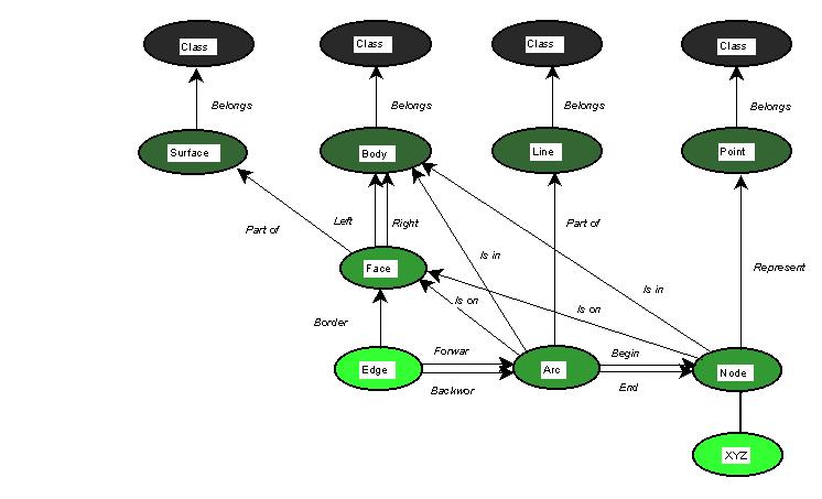
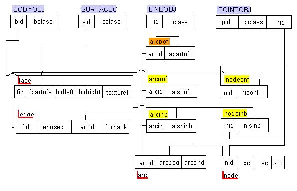
Figure 5-3: 3D FDS: logical model
The fundament of 3D FDS is the concept for a single-valued map, i.e. a CnsO (node, arc, face or edge) can appear in the description of only one GO of the same dimension (Molenaar 1989). The idea of the single-valued approach is to partition the space into non-overlapping objects (0,1,2,3 D), and thus ensuring 1:1 relationships between GO and CnsO of same dimensions, e.g. surfaces and face. CnsO of different dimensions can overlap, e.g. relationships node-on-face, arc-on-face, node-in-body and arc-in-body are explicitly stored.
The last basic concept is related to linking thematic class and geometry. Convention 2 imposes a thematic class to have instances GO of only one type, as the belonging to a class is compulsory (convention 1).
The model (see Figure 5-2) is mapped into a relational data model (Rikkers et al. 1993) and extended by Tempfli and Pilouk 1996 for texture storage. The mapping leads to 13 normalised tables (see Figure 5-3). The research reported currently has approved 3D FDS as appropriate for modelling and analysis of urban data. This section discusses the model with respect to the visualisation strategy presented in Chapter 3 (see also Zlatanova and Tempfli 1998).
In general, 3D FDS contains all the necessary data to visualise the geometry of objects. As mentioned, VRML (and the most of the rendering packages) operate with faces (triangles), which are represented by vertexes. The model also provides the orientation of faces, which is crucial for the correct rendering. Since the model has well defined objects, it can be extended with information about geometric attributes and behaviour. The disadvantages of the model focus on mainly performance issues. Since the performance is influenced by a particular implementation, the following analysis is based upon the relational mapping (see Figure 5-3).
The first concern raises from the lack of explicit relationship face-part-of-body, which has impact on 1) the response time and 2) the size of the database. One of the basic visualisation queries, i.e. "find all the faces composing a body" requires a double check, i.e. the fields bodyleft and bodyright has to be visited for each record. The size of the database may grow rapidly due to storage of repetitive information for some objects. For example, terrain data represented by TIN have an air body (0) to the left and an underground body (-1) to the right (see Table 5-3).
Table 5-3: An example of terrain data stored in the FACE table
|
|
|
|
|
|
|
|
|
|
|
|
|
|
|
|
|
|
|
|
|
|
|
|
|
|
|
|
|
|
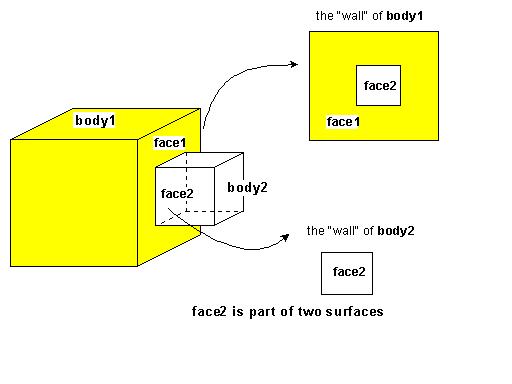
The second concern is the organisation of texture. In general, one object (body or surface) can be textured with one or several images by texture mapping, and one image file can be used to drape several faces (see Chapter 4). 3D FDS is capable of keeping one or more textures per face. The textures can be single images or part of one image. Sithole 1997 proposes several different methods for storage of texture in order to facilitate dynamic loading of images from the database. One of the methods, i.e. the composition of textures needed for a surface in one image file, suits the VRML concepts (see Chapter 4). However, it is still impossible to wrap a surface or a body with one image file or to texture the face (or both its sides) with different textures. In many cases, draping with one image file is much more efficient, e.g. terrain. An indication as to which side of the face is textured might be necessary as well, e.g. two adjacent buildings with a common wall. This is a quite important issue for dynamic modelling: suppose the user wishes to see only body2, which has a common wall with body1, constituted of face1 and face2, then the wall of body2 has to have the appropriate texture (see Figure 5-4).
Figure 5-4: An example of a face needing two textures
The fourth concern is the explicit storage of the relationships node-on-face and arc-on-face. These relationships may easily create a false impression of "sinking" in or "flying" over the face during rendering. 3D FDS allows faces with an arbitrary number of arcs, but requires their planarity. Forcing the nodes to lie exactly on a plane can ensure the planarity. The approach, however, raises a number of questions about the computation of the approximate plane, the method of node projection on the plane, the preservation of the relationships, etc., which require more investigations. The simpler method is triangulation of the face and converting it into a surface. The triangulation can be executed prior to creating the VRML document, or left to the VR browsers. Now suppose a node or an arc lies inside the face and the face is independently triangulated, a variety of "arty-facts" (e.g. an arc flying over the face, an arc crossing the face, a node below or above the face) may be observed on the screen. Pitfalls (blinking and disappearing while navigating) are observed even if the face is strictly planar and the arc lies exactly on it. Therefore, existing arcs-on-face and nodes-on-face have to be incorporated in the triangulation of the face. Since this cannot be left to the browser, intermediate algorithms are required for triangulation and control of these relationships.
The last concern is the visualisation of holes in faces. Although permitted, holes do not have a special indication in 3D FDS. Holes are stored together with the parent face, as the arcs bordering a hole have an opposite to the arcs bordering the face direction. Clearly, the holes can be recognised, as the necessary order can be obtained by checking the arcend/arcbegin relationship per arc in the ARC table. This operation, however, has to be performed for each arc bordering a face, which requires more sophisticated and thus slower algorithms for data extraction.
In summary, 3D FDS supplies sufficient data for rendering, and can be easily extended to accommodate data about behaviour and geometric attributes. However, the time for creating VRML documents is expected to be rather long due to the following conceptual characteristics:
TEN was introduced by Pilouk (see Tempfli and Pilouk 1994 and Pilouk 1996) to overcome some difficulties of 3D FDS in modelling objects with indiscernible boundaries. According to the definitions, TEN has four constructive objects (tetrahedron, triangle, edge, node). The relationship arc-node is given by the ARC table; the TRIANGLE table contains the tetrahedron-triangle-edge link. A body object is composed of tetrahedrons, a surface object of triangles, a line object of arcs and a point object of nodes. The general rule for creating the model is based on the fact that each node is part of an arc, each arc is part of a triangle and each triangle is part of a tetrahedron (see Figure 5-5 and Figure 5-6). Singularities are not permitted. The model is appropriate for representing irregularities in the real world, such as terrain, soil, air, geological objects, etc. 3D man-made objects are embedded as 3D FDS features in TEN (see Pilouk 1996). Since the model uses the simplex-complex concept (see Egenhofer and Herring 1992), TEN can be expected to cover the scope of possible topological relations in 3D space. Pilouk 1996 reported series of positive results concerning the construction of the model.
Figure 5-5: TEN: n-dimensional conceptual model
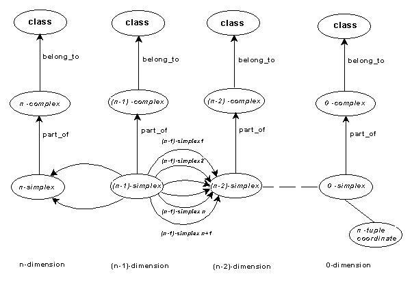
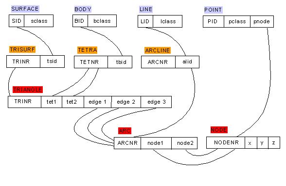
Figure 5-6: TEN: logical model for n=3
The model furnishes the data needed for display of graphic information in the most appropriate way, i.e. triangles. In this respect, TEN is perhaps the optimal model for visualisation of surfaces and irregular bodies. Maintenance of triangles solves a couple of visualisation problems mentioned regarding 3D FDS, i.e. holes and pitfalls due to explicit storage arc-on-face and node-on-face. Parsing of the VRML file must be faster due to the provision of only triangles for rendering, i.e. the VR browser does not need to perform a triangulation. Volume and area computations are facilitated as well.
Considering the logical model, data to create a VRML document can be extracted in several steps, applying SQL statements and the host language. Suppose during the construction phase, edge1, edge2, and edge3 are oriented in an anti-clockwise direction (for surface triangles of the body), the order of the nodes still has to be derived. Therefore the steps to extract triangles for VRML visualisation might be:
SELECT TETNR FROM TETRA WHERE tbid=OBJECT
For each TETNR do {
SELECT n11, n12 FROM TRIANGLE, ARCNR
WHERE TETNR=tet1 and tet2=0 and edge1=ARCNR;
SELECT n21, n22 FROM TRIANGLE, ARCNR
WHERE TETNR=tet1 and tet2=0 and edge2=ARCNR;
(Note, that a body has a number of invisible triangles that do not need to be visualised. Assuming that the "air" body has ID=0 and tet2 is the right body than the condition tet2=0 will extract only the visible triangle. Edge3 is not necessary because all the nodes are extracted.)
Order the nodes:
If (n12=n21) the order is n11, n12
(n21), n22
If (n12=n22) the order is n11, n12
(n22), n21
If (n11=n21) the order is n12, n11
(n21), n22
If (n11=n22) the order is n12, n11
(n22), n21
For each NODE
do {
SELECT x, y, z FROM NODE WHERE NODE=NODENR;
}
}
A number of undesirable side effects concerning the VRML creation may occur. First, the VRML document may become rather long due to more faces in the description section. The VRML node IndexetFaceSet may preserve the size of the co-ordinate list (the number of nodes can be the same for 3D FDS and TEN); however, the list of the triangles given in IndexCoord will at least double. The increase depends on the shape of the real objects and more specifically on the roofs of the buildings. While buildings with complex roof construction (represented by many triangles in 3D FDS) will be affected only with respect to the walls, flat roofs with many corners will create a lot of triangles. This may slow down the delivery of data to the client station.
Second, since the space is completely subdivided into tetrahedrons, the interiors of objects (e.g. buildings), as well as the open space, are also decomposed into tetrahedrons. These tetrahedrons, however, disturb the scene and have to be omitted from the VRML document, which requires additional algorithms to be developed. The covering surface of a body (needed for visualisation) can be either stored in the database as an independent object, or created on the fly by an algorithm selecting the faces of a body, which are not interior. The first approach will lead to database size expansion, the second one will cause longer response time.
Figure 5-7: A simple box represented in 3D FDS and TEN
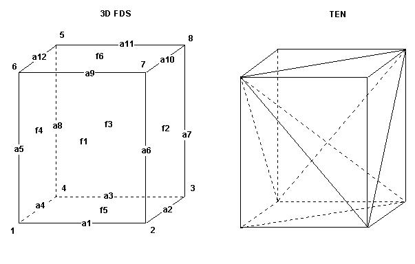
TEN maintains two more tables, i.e. TETRA and TRISURF, which are necessary to compose the needed complex. The size (144 bytes for the example) is such to "compensate" 3D FDS for the more expensive face-arc relationship. That is to say, FACE+EDGE (3DFDS) needs less space (408 bytes) than TETRA+TRISURF+TRIANGLE (TEN) (576 bytes).
The significant in data is a result mostly of the large number of arcs and triangles obtained from the full triangulation. A subdivision of a face bordered by n-arc (n>3) leads to (n-3) additional faces and (n-3) new arc. For example, the ARC table in TEN contains more records than the one in 3D FDS. The increase is at least as much as the number of the rectangular faces plus at least one internal arc. The growth of information is even faster for faces with holes, as the rate depends on the number of holes. The image pieces used for texturing also have to be subdivided and we face again an increase of data: triangular pieces of texture require larger storage space.
Last, is still difficult to create an urban spatial model it in TEN, mostly because of a lack of efficient algorithms for constrained tetrahedronization.
|
|
|
||||||
| Number | b/r | Bytes | Number | b/r | Bytes | ||
| Bodyobj | 1 | 24 | 24 | Body | 1 | 24 | 24 |
| Surfobj | 1 | 24 | 24 | Surface | 1 | 24 | 24 |
| - | 0 | 0 | 0 | Tetra | 6 | 8 | 48 |
| - | 0 | 0 | 0 | Trisurf | 12 | 8 | 96 |
| - | 0 | 0 | 0 | ||||
| Face | 6 | 16 | 96 | Triangle | 18 | 24 | 432 |
| Edge | 24 | 13 | 312 | - | 0 | 0 | 0 |
| Arc | 12 | 12 | 144 | Arc | 19 | 12 | 228 |
| Node | 8 | 16 | 128 | Node | 8 | 16 | 128 |
| Total | 50 | 57 | 680 | Total | 65 | 116 | 980 |
The spatial model introduced by Brisson 1990 and extended by Pigot (see Pigot 1992) will be referred to as the tuple model. It defines cells and cell complexes upon the fundamental properties of a manifold. A k-cell (where k is the dimension of the cell) is defined as a bounded subset of a k-manifold and hence it is homeomorphic to a k-manifold with (k-1)-manifold boundary(s). The k-cell complex is the union of all the k-dimensional and lower cells. Some later extensions (see Mesgari et al 1998) of the model permit the existence of singular n-cells, e.g. 0-cell inside 2-cell, 2-cell inside 2-cell (holes), 3-cell inside 3-cell (tunnels). Under these circumstances, any spatial object is described as a set of tuples of 3-cell, 2-cell, 1-cell and 0-cell, i.e. the representation of cells is implicit. From construction point of view, the model permits cells with an arbitrary shape. For example, the box above does not require decomposition into tetrahedrons. Despite less partitioning, the model does not lead to fewer records. For example, face f1 (see Figure 5-7), part of a body b1, will be represented by 16 records (see Table 5-5) and body b1 is fully described by 96 records. According to the author's estimation, complex real objects may lead to enormously large representations (see Pigot 1995).
| Records | 1 | 2 | 3 | 4 | 5 | 6 | 7 | 8 | 9 | 10 | 11 | 12 | 13 | 14 | 15 | 16 |
| 0-cell | 1 | 1 | 1 | 1 | 2 | 2 | 2 | 2 | 7 | 7 | 7 | 7 | 6 | 6 | 6 | 6 |
| 1-cell | 1 | 1 | 5 | 5 | 6 | 6 | 1 | 1 | 9 | 9 | 6 | 6 | 5 | 5 | 9 | 9 |
| 2-cell | 1 | 1 | 1 | 1 | 1 | 1 | 1 | 1 | 1 | 1 | 1 | 1 | 1 | 1 | 1 | 1 |
| 3-cell | 1 | 0 | 1 | 0 | 1 | 0 | 1 | 0 | 1 | 0 | 1 | 0 | 1 | 0 | 1 | 0 |
The model promises 1) the capacity to provide a large spectrum of topological relations between cells and complex cells, 2) easy implementation (a table structure), and 3) an easy maintenance, due to the claimed solid mathematical foundations. Reports on investigations of the model for a variety of applications are already available (see Mesgari et al 1998, Raza and Kainz 1998).
Since the construction rules are similar to the rules of 3D FDS, the model can be considered quite suitable for modelling in urban areas. In the visualisation respect, the extraction of faces and points (needed for VRML documents) seems to be a simple operation, due to the explicitly stored link between the cells. The data obtained from the tuple representation, however, lacks any indication regarding the order. Supplementary records are needed to establish the order (clockwise or anti-clockwise) of cells (note the cyclicity is ensured). This will result in further increase of the space for database storage and eventual complication of the algorithms for data extraction. The performance is difficult to evaluate without implementation. Assuming a relational implementation, the entire tuple information is available in one relational table, which has advantages and disadvantages. On one hand, there is no need to perform JOIN operations to select data for VRML document. On the other hand, the size of the table grows tremendously, which slows down the speed of SELECT operations. For example, the records for the box above occupy 1536 bytes storage space, which is double compared with 3D FDS (see Table 5-4).
It is apparent that TEN and 3D FDS permit more compact representations than the tuple model. Note also that an appropriate JOIN operation can create the tuple table from TEN. 3D FDS can be converted into a tuple table as well, if special operators process the explicit relationships node-on-face, node-in-body, arc-on-face and arc-in-body. The opposite conversion is possible with some additional operations, i.e. partitioning of the objects according to the construction rules of TEN, and creation of new tables for singular cases in 3D FDS.
Among the three spatial models, 3D FDS and the tuple model reveal advantages for 3D modelling: 1) the shape of the real objects is maximally preserved, 2) complete subdivision of the space is not required and 3) many singularities (e.g. holes, node-on-face, arc-on-face) are permitted. More elaborated discussion on space subdivisions and singularities is given in Section 5.5.2. A simple comparison of size representation indicates some advantages of 3D FDS. TEN is quite appropriate for visualisation with respect to avoiding visualisation artefacts, but requires large storage space and imposes undesirable partitioning of real objects from urban areas. The tuple model leads to the largest representation among the three models. Bearing in mind the expected amount of data in urban models, its utilisation might result in an unmanageable system.
Clearly, advantages of a model in one of the aspects occur as disadvantages in another aspect (see Table 5-6), which motivates the search for alternatives. Alternatives can be found in altering both construction rules and objets. Although quite approximate, the estimation of the models reveals benefits in utilising 3D FDS. The weak aspect of 3D FDS is visualisation, which, however, can be improved if more strict construction rules are applied. Let us introduce the rule "all the faces are triangles" and analyse the new model denoted 3D FDS (triangulated). The partition of the objects will be indeed higher, all the surfaces have to be triangulated, however the space subdivision is unchanged. Singularities will be relatively reduced, i.e. the relationships node-in-body and arc-in-body will remain but node-on-face and arc-on-face will disappear. These changes will result in a new logical model. The fields of the EDGE table will become a constant number, which will reduce the size of the table significantly. Calculations of the database size indicate that the modified structure of the relational table will compensate for the increased number of triangles in 3D FDS (triangulated). In general, 3D FDS (triangulated) promises greater suitability for our system architecture than 3D FDS.
| Aspects | Criteria | 3DFDS | TEN | The tupple
Model |
3DFDS
(triangulated) |
| Modelling | Partition | 1 | 3 | 2 | 2 |
| Subdivision of space | 1 | 3 | 1 | 1 | |
| Singularities | 1 | 3 | 1 | 2 | |
| Visualisation | Faces and co-ordinates | 1 | 1 | 1 | 1 |
| Orientation of faces | 2 | 1 | 3 | 1 | |
| Artefacts | 2 | 1 | 2 | 1 | |
| Performance | Time for database traversal
and VRML creation |
3 | 2 | 3 | 1 |
| Time for delivery | 1 | 3 | 1 | 2 | |
| Time for parsing | 1 | 2 | 1 | 1 | |
| Database size | 1 | 2 | 3 | 1 | |
| Total |
1-good, 2-acceptable, 3-unsatisfactory
Spatial models in 2D GISs commonly maintain three constructive primitives, i.e. nodes (0-cell), arcs(1-cell) and faces (2-cell). The topology is defined by explicit or implicit neighbourhood information between all the CnsO. Spread over all the objects in the entire map (or layers of different maps), the topology allows spatial analysis of various complexities to be carried out. Usually, the arc is the basic constructive object, mainly because it provides a finite boundary and co-boundary information. The arc has two bounding nodes and two co-bounding faces that strictly define the neighbourhood of the arc. A constructive object with the same properties does not exist in 2D space. The node lacks bounding CnsO, and the face does not have a co-bounding CnsO. In addition, the relation node-arc and face-arc is one-to-many. Several spatial models have been built utilising the unique properties of the arcs. Early approaches such as the DIME model (see Corbet 1975) store the two nodes bounding an arc and its co-bounding polygons (faces). To speed up the retrieval of faces, later spatial models explicitly store the boundary of the face usually as a list of arcs. Examples are the arc-node model described by Aronoff in 1989 (see Aronoff 1995), FDS (see Molenaar 1989), ATKIS (Hesse and Leahy 1990), etc.
Early spatial models in computer graphics systems (CAD) make use of the same three CnsO. Since the topology in computer graphics is defined for the surface of a solid object, many of the spatial models are in a sense similar to those in GIS. Despite the different original mathematical reasoning, they can be classified as subdivisions of 2-manifolds (see Chapter 2). A study on existing modelling systems, which operate with solids presented by Baer et al in 1979 has revealed that the arc (edge) is the key constructive element of many systems. The very first structuring for graphic visualisation purposes is the winged-edge model proposed by Baumgart in 1974 (see Mäntylä 1988). The model maintains information about the left and right faces, and left, right, counter and clockwise arcs of an arc. Following this model, several graphic systems have been developed, e.g. Geomed, Geomap and Build-2 (see Baer et al 1979). Several systems have a structure similar to the 2D GISs mentioned above, i.e. face is represented as a list of arcs and arc is represented as a list of nodes (e.g. PADL, BUILD, COMPAC, PADL). However, two modelling systems (among 11 explored) have been organised on the relation between only faces and nodes (i.e. the faces are represented by lists of nodes), one maintains only faces with neighbouring faces and two have expressed faces as lists of arcs and lists of faces. One of the systems missing arcs is EUKLID, developed at LIMSI, Orsay, France in 1976. Each body is represented by a list of faces with information about the number of the nodes in a face and the pointer to the first node in a face. All the descriptions of faces are stored in a file called "line". The nodes are in a separate file "vertices" as current positions of nodes in the file are used as ID to complete the description of faces. The system has been capable of operating with several primitives, e.g. box, wedge and polyhedron, as well lines and points. Although the study is from the time of vector graphics, it is evidence that graphics systems based on faces and nodes has been successfully realised in the past.
Currently, the status of arc in CG is more doubtful than ever. On one hand, the requirements of VR systems for real-time visualisation and effective management of large volumes of spatial data have directed the research in CG toward investigation of hierarchical data representations with minimal CnsO for storage (see Campagna et al 1999, Lindstrom et al 1996, Popovich and Hoppe 1997). On the other hand, the standard rendering engines, e.g. OpenGL (see Woo et al 1997) and Direct 3D, which are already widely hardware implemented, contain sets of procedures that require vertices ordered in a special manner. The structure of data in VRML lacks arcs too (see Chapter 4).
The function of arcs in 3D FDS is basically representation of the link between nodes and specification of the order (in contrast to the 2D variant). Further, the arcs are building elements for lines and edges, where the order is explicitly specified or can be specified. If arcs do not exist, the line object and edge CnsO can be represented by a sequence of nodes. The replacement of sequence of arcs by sequence of nodes in the LINE and EDGE tables will not increase the number of records drastically: it remains the same in the EDGE table and increases by one per line in the LINE table. Consequently, the global effect of this modification of the model will be the significant reduction of data. The ARC table is one of the largest tables. The results of experiments with triangulated surfaces shows that the ratio faces:arcs:nodes is 2:3:1. With the elimination of the ARC table, the relationships arc-in-body and arc-on-face are also superfluous, because node-in-body and node-on-face will represent the same spatial relationships.
On the basis of the discussion above, we have created the hypothesis that arcs can be safely omitted from the representation of the model. To prove the hypothesis a new spatial model will be defined in the next section. Since the model was inspired during the experiments with 3D FDS, some principles are quite similar. The concepts of the 3D FDS that are preserved in the new model will be explicitly mentioned.
5.5 The Simplified Spatial Model (SSM)
In this section, the definition of a new spatial model will be given. It will be referred to as Simplified Spatial Model because arcs are not used to construct objects. According to the proposed definition of an object, the geometry of each spatial object can be associated with four abstractions of geometric objects, i.e. point, line, surface and body. A point is a spatial object that does not have shape or size but position is the space. A line is a type of a spatial object that has length and position. A surface is an abstraction of spatial object that has position and area. A body is a type of spatial object that has a position and a volume. All the GO are built of smaller, simpler elements, i.e. constructive objects. The model consists of two CnsO, i.e. node and face.
The formal definition of the spatial model establishes
the rules according to which an object can be composed, clarifies allowed
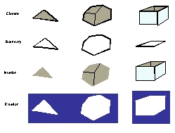
configurations and specifies the topological primitives (closure,
boundary,
interior
and exterior) needed for the later elaboration on neighbourhood
relations. Furthermore, we assume that all the objects are embedded in
Euclidean
3D-space, denoted by IR
n where ![]() .
The formalism employs fundamental definitions, theorems and concepts of
set theory (see Lipschultz 1964 and Willard 1970) and linear algebra (Anton
1994). The basic category utilised in the definitions is the one of indexed
sets. The index gives a unique identification of any spatial object,
which facilitates many stages of the implementation (see Chapter
7).
.
The formalism employs fundamental definitions, theorems and concepts of
set theory (see Lipschultz 1964 and Willard 1970) and linear algebra (Anton
1994). The basic category utilised in the definitions is the one of indexed
sets. The index gives a unique identification of any spatial object,
which facilitates many stages of the implementation (see Chapter
7).
5.5.1 Definition of constructive objects
Let U be the universe and p any point in it.
Definition 1: The node denoted by Ni is an indexed set of one element p, i.e.:
![]() , where i
is the unique index of a node,
, where i
is the unique index of a node,
with the following property:
a) Two nodes cannot have the same element,
i.e. they are always
disjoint:
If![]() is a point
from
IR
nsuch
is a point
from
IR
nsuch ![]() and
and![]() , then
, then ![]() and
and ![]()
The interior of a node, denoted by N°,
is the empty set. The boundary of the node, denoted by ¶ N,
is the node by itself. The closure of a node, denoted by`N,
is the union of the boundary and the interior, i.e. ![]() .
The exterior of a node, denoted by N¯, is the difference
between the universe U and the closure of`N, i.e.
.
The exterior of a node, denoted by N¯, is the difference
between the universe U and the closure of`N, i.e. ![]() .
.
A node embedded in IR3 is represented by a point with co-ordinates (x,y,z). It is not necessary for all the points in IR 3 to be nodes. One can think about a building where only the footprints have known co-ordinates and thus only they are represented in the model as nodes. The geometric representation of the exterior of a node is everything but the node by itself.
Next, we will define the family set of all the nodes ND,
which belong to the same topological space. ND is a subset of all the points
in the universe, i.e. ![]() .
.
Definition 2: If ![]() is
the topological space then the set of all the n nodes
is
the topological space then the set of all the n nodes![]() is
denoted by ND, i.e.
is
denoted by ND, i.e.
![]()
with the following properties:
a) The intersection of all the nodes
is the empty set, i.e.![]() , i.e.
the subsets Ni are a partition of ND.
, i.e.
the subsets Ni are a partition of ND.
b) Two nodes ![]() and
and![]() in IR 3 are
connected
iff there is a straight line linking them, otherwise they are disconnected.
The straight line connecting two nodes will be referred to as link in
the following text.
in IR 3 are
connected
iff there is a straight line linking them, otherwise they are disconnected.
The straight line connecting two nodes will be referred to as link in
the following text.
Definition 3: A face
denoted by F is an indexed set of x ordered nodes![]() ,
where
,
where ![]() (if
x = 3
the face is called triangle), i.e.
(if
x = 3
the face is called triangle), i.e.
![]() ,
,
where f is the face index of a node specifying the current order in a face Fj,
with the following properties:
(for simplicity, the unique index i is omitted)
a) Fj
is a connected set for each ordered pair![]() ,
, ![]() .
.
b) In the set of nodes cannot exist
two equal nodes, i.e. the intersection of the nodes ![]() is
the empty set, i.e.
is
the empty set, i.e. ![]() .
.
c) Each triple of nodes![]() ,where
,where ![]() and
and ![]() fulfils
only one planar equation
fulfils
only one planar equation ![]() in
IR
3,
i.e. the face is planar .
in
IR
3,
i.e. the face is planar .
d) There is at least one ordered triple
of nodes![]() , which does not fulfil
the line equation
, which does not fulfil
the line equation![]() in IR 3.
in IR 3.
e) All the nodes ![]() ,
, ![]() are
anti-clockwise oriented in IR3, e.g.. for each ordered
triple
are
anti-clockwise oriented in IR3, e.g.. for each ordered
triple ![]() ,
, ![]() which
have a planar equation
which
have a planar equation ![]() and
a normal vector n=(a,b,c), the constant
and
a normal vector n=(a,b,c), the constant ![]() .
.
f) F is convex in IR
3,
i.e. if ![]() are three points
such that
are three points
such that ![]() then for each
ordered triple
then for each
ordered triple ![]() the
angle
the
angle ![]() ,
,![]() and
and ![]() is
is![]() .
.
g) The set of nodes ![]() is a subset of the boundary of the face, i.e.
is a subset of the boundary of the face, i.e.![]() .
.
The interior of F, denoted by F°,
is the area closed by the set of nodes. The boundary of F, denoted
by ¶F is the union of all the connected nodes ![]() ,
i.e.
,
i.e.
![]()
The closure of F, denoted by`F,
is the union of the boundary ¶F and the interior F°,
i.e. ![]() . The exterior
of F, denoted by F¯ is the set difference of the universe
U and the closure`F,
i.e.
. The exterior
of F, denoted by F¯ is the set difference of the universe
U and the closure`F,
i.e.
![]()
Definition 4: The family
set of all the m faces![]() is denoted by FC , i.e.
is denoted by FC , i.e.
![]() ,
,
where j
is an unique index of a face, with
the following property:
a) The intersection of all the faces
is the empty set, i.e. ![]()
, i.e. the subsets Fj are a partition
of FC. This means that there are not two equal faces.
The two constructive objects may interact with each other
while representing real objects. To resolve some of the obstacles discussed
in the previous section, the interactions between the CnsO are specified
in the following statements:
b) A node ![]() and
a face
and
a face![]() are disjoint, if
the intersection of the node with the nodes
are disjoint, if
the intersection of the node with the nodes![]() is
the empty set, i.e.
is
the empty set, i.e. ![]() . Otherwise
the node
. Otherwise
the node![]() is part of the
face
is part of the
face![]() .
.
c) Two faces are disjoint if
for each pair of nodes ![]() ,where
,where![]() and
and ![]() their
intersection is the empty set, i.e.
their
intersection is the empty set, i.e. ![]() .
.
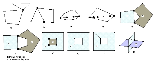
Figure 5-10: Subdivisions of a face with a node
Configuration e) to Definition 2b,
i.e. the link between the nodes is not a straight line
Configuration f) to Definition 3f
and Definition 4c, i.e. face f2 is not convex and the
intersecting nodes are not in sequential order for f2
Configuration g) to Definition 3g,
i.e. there are nodes in the interior of face f1
Configuration h) to Definition 3a,
i.e. the boundary of face f1 is disconnected
Configuration i) to Definition 3f,
i.e. face f1 in not convex
Configuration j) to Definition 4c,
i.e. the order of the intersecting nodes is not sequential for either of
the faces.
The definitions of CnsO introduced above differ from those given for a face in 3D FDS. The additional restrictions to the shape of the faces (convex and without holes), and the elimination of the relation node-on-face by subdividing the face, ensure correct visualisation in any rendering package or VR browser.
5.5.2 Definition of geometric objects
The two constructive objects are now used to compose the four geometric objects, i.e. point, line, surface and body. The geometric objects consist of only one type of CnsO, as follows: points and lines consist of nodes and surfaces and bodies are built of faces. This section gives formal definitions and specifies the properties of GO. The possible relations between GO and CnsO and the rules to construct topology, which can be derived from the definitions, are discussed.
Definition 5:
A
point
denoted by Pk is an indexed set of p nodes Ni,
where p = 1 i.e.:
![]() ,
,
where p is the point index of the node.
The topological primitives of a point are:
Definition 6:
If ![]() is
the topological space, then the family set of all the pn points
is
the topological space, then the family set of all the pn points![]() denoted
by PT is:
denoted
by PT is:
![]()
and has the following properties:
a) The intersection of all the points
is not equal to the empty set, i.e. ![]() ,
i.e. the subsets Pk are not a partition of PT.
This
means that the existence of two equal points is possible.
,
i.e. the subsets Pk are not a partition of PT.
This
means that the existence of two equal points is possible.
b) Two points ![]() and
and ![]() are
disjoint
if the intersection of the nodes composing the points
are
disjoint
if the intersection of the nodes composing the points ![]() and
and ![]() is
the empty set, i.e.
is
the empty set, i.e. ![]() .
.
c) For some![]() a
set of points
a
set of points ![]() can exist
such that
can exist
such that ![]() ,..,
,.., ![]() .
This means that the points
.
This means that the points ![]() are
equal.
are
equal.
d) ![]() ,
i.e. there are nodes, which does not constitute a point.
,
i.e. there are nodes, which does not constitute a point.
e) For some point ![]() a node
a node![]() can exist such that
can exist such that ![]() ,
, ![]() .
This means that the point
.
This means that the point ![]() meets
the
face
meets
the
face![]() . Otherwise the point
. Otherwise the point ![]() and
the face
and
the face![]() are
disjoint.
are
disjoint.
f) a point ![]() can be a subset of the boundary of a face
can be a subset of the boundary of a face![]() ,
i.e.
,
i.e.![]() .
.
According to the definitions above, several points can have a common node and thus they are equal. Points can coincide with the boundary of a face but not with the interior. Similar to the case node-in-face, the face must be subdivided. Compare with 3D FDS the difference is the multi-valued concept, i.e. one node can constitute more than one point object.
Definition 7:
A
line denoted by Lk is an indexed set of x nodes
NI, ![]() ,
i.e.
,
i.e.
![]() , where l
is
the line index of a node,
, where l
is
the line index of a node,
with the following properties:
a) There is one pair of sets denoted
by first node![]() and last node
and last node![]() ,
which are disconnected.
,
which are disconnected.
b) The line is closed iff ![]() .
.
c) L is a connected set for
each ![]() , where
, where ![]() .
.
d) The intersection of each pair of
nodes![]() ,
, ![]() is
the empty set, i.e.
is
the empty set, i.e. ![]() .
.
e) Lines are homeomorphic to a 1-manifold,
i.e. they are simple lines.
Definition 8:
If ![]() is
the topological space, then the family set of all the ln lines
is
the topological space, then the family set of all the ln lines![]() denoted
by LN is:
denoted
by LN is:
![]() ,where k
is
the unique index of a line,
,where k
is
the unique index of a line,
and has the following properties:
a) The intersection of all the lines
is not equal to the empty set, i.e. ![]() ,
i.e. the subsets Lk are not a partition of LN.
This
means that the existence of two equal nodes in a line is
possible.
,
i.e. the subsets Lk are not a partition of LN.
This
means that the existence of two equal nodes in a line is
possible.
b) The line ![]() and
the node
and
the node ![]() are disjoint
iff
the intersections of the node with the nodes of the line
are disjoint
iff
the intersections of the node with the nodes of the line ![]() is
the empty set , i.e.
is
the empty set , i.e. ![]() ,
where
,
where ![]() , otherwise the node
is part of the line.
, otherwise the node
is part of the line.
c) The line ![]() is
disjoint
from the face
is
disjoint
from the face ![]() iff the intersections
of each pair of nodes
iff the intersections
of each pair of nodes ![]() ,
where
,
where ![]() and
and ![]() is
the empty set , i.e.
is
the empty set , i.e. ![]() ,
where
,
where ![]() .
.
d) The line![]() stronglymeets
the
face
stronglymeets
the
face![]() iff for some line
iff for some line ![]() there
is a set of nodes
there
is a set of nodes![]() such that
such that ![]() ,
, ![]() .
If the set intersection of nodes contains only one element
.
If the set intersection of nodes contains only one element![]() ,
then the line
,
then the line![]() weaklymeets
the
face at
weaklymeets
the
face at![]() .
.
e) A line![]() cannot be a subset of the interior of a face
cannot be a subset of the interior of a face![]() ,
i.e. the nodes
,
i.e. the nodes ![]() constituting
the line can be part of the boundary of the face
constituting
the line can be part of the boundary of the face ![]() .
The property follows from the definition of a line and the property g)
in Definition 2 (the Proof is similar
to Definition 3.e). The face has to be subdivided into
smaller faces to incorporate the line (see Figure
5-12).
.
The property follows from the definition of a line and the property g)
in Definition 2 (the Proof is similar
to Definition 3.e). The face has to be subdivided into
smaller faces to incorporate the line (see Figure
5-12).
f) ![]() ,
i.e. there are nodes, which does not constitute a line.
,
i.e. there are nodes, which does not constitute a line.
Figure 5-12: Subdivisions of a face with a line
The line in the model is restricted to laying only on the boundary of a face or to existing freely in the space. If a line has to cross a face, then the face must be subdivided (or triangulated) in such a way as to include the line (see Figure 5-12).
Faces compose the next two geometric objects. Since the faces are set of nodes, some statements will refer to the nodes of the faces. To distinguish between any nodes and nodes part-of-face, the corresponding unique and face index of nodes will be utilised.
Definition 9:
A
surface
denoted by Sk is an indexed set of x faces Fj,![]() ,
i.e.
,
i.e.
![]() , where s
is
the surface index of a face
, where s
is
the surface index of a face
with the property that the nodes in a surface Sk,
i.e.![]() belong
to either one or two faces, part of the surface, i.e.
belong
to either one or two faces, part of the surface, i.e.
a) If the intersection of a pair of
nodes![]() and all the other pairs
of nodes is the empty set, i.e.
and all the other pairs
of nodes is the empty set, i.e. ![]() ,
where x1 is the number of faces in a surface and x2 is the number
of nodes in a face, then the pair of nodes
,
where x1 is the number of faces in a surface and x2 is the number
of nodes in a face, then the pair of nodes![]() belong
to only one face. If the set of nodes is equal to the empty set , i.e.
belong
to only one face. If the set of nodes is equal to the empty set , i.e. ![]() .
.
b) If the intersection of a pair of
nodes![]() and all the other pairs
of nodes differ the empty set, i.e.
and all the other pairs
of nodes differ the empty set, i.e. ![]() ,
then the pair of nodes
,
then the pair of nodes ![]() belong to two faces. If all the pairs of nodes belong to two faces then
the surface is a closed surface.
belong to two faces. If all the pairs of nodes belong to two faces then
the surface is a closed surface.
c) Surfaces are homeomorphic to 2-manifold,
i.e. they are simple surfaces.
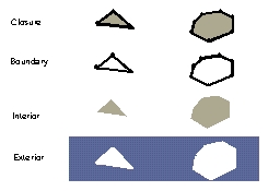
d) The topological primitives of a
surface are:
Figure 5-13: Closure, boundary, interior and exterior of a surface
According to 3D FDS, bodies are constructed on the basis of the existing faces, i.e. each face is part of two bodies. If a face closes part of space in an existing body, then a new body is created. The weakness of the approach is basically in the modelling and maintenance of bodies. For example, a building constructed of two floors (represented as a box with a face in the middle) needs two bodies for the space subdivided by the floors. Thus the building, which most probably has to be maintained as one object, has to be separated into two geometric objects (i.e. two new ID of bodies). A number of operations on geometric and thematic information will be needed to hide the modification from the user.
TEN suggests a more elaborate solution, i.e. each body, regardless of the shape, is subdivided into tetrahedrons. The benefit is that the geometric object remains one object, independent of the geometric changes. The example of a building with floors modelled in TEN will require new tetrahedrons. The ID of the object, however, will be preserved. As discussed before, the disadvantages of TEN are related to the partition of the open space and the database size.
A third approach, i.e. maintenance of singularities, is reported for the cell model (see Mesgari et al 1998). The 3-cell (i.e. body) can contain 3-cell, 2-cell, 1-cell and 0-cell, i.e. no construction rules for the subdivision of the body are imposed. The modelling of the interior of the body is the responsibility of the user. It is well known that singularities permitted in the model allow users to preserve the variety of isolated objects of the real world, e.g. a room in a building, a counter in a building, a desk in a room, a lamp on a desk, a decoration wall in a building. However, the approach reveals disadvantages in several directions: 1) the duplication of data is inevitable, 2) the retrieval and updating require more sophisticated operations and 3) the consistency check is more complicated.
In short, singularities are convenient for the user and the modelling process but complicate the retrieval and control of data, and vice-versa, i.e. the partitioning eases the maintenance of data and imposes constructive rules (mostly undesirable) on the reconstruction. Apparently, some balance between advantages and disadvantages has to be established with respect to the application of the spatial model. The spatial model introduced here aims at visualisation and spatial analysis in urban areas. The definitions presented so far forbid singularities for 1D and 2D objects, i.e. node or point on line, node or point on face, line on face. Thus the first part of the requirements if fulfilled: the models ensure correct visualisation, i.e. provision of data that cannot cause artefacts and rendering problems. Consequently, 0D, 1D and 2D objects have to obey strict constructive rules. The subdividing rules of the body will not further affect the visualisation because the body has an optimal representation for rendering, i.e. a set of faces. Thus the partition of 3D objects is significant for the re-construction and completion of spatial analysis. The discussion above motivates a few singularities, i.e. face-in-body and node-in-body, to favour the modelling process and spatial analysis. Since the objects inside the body cannot be detected from the definition of body, the relations will be explicitly stored in the model.
Definition 12:
If ![]() is
the topological space the family set of all the bn bodies
is
the topological space the family set of all the bn bodies![]() denoted
by BD is:
denoted
by BD is:
![]() ,where k
is unique body index
,where k
is unique body index
and has the properties:
a) The intersection of all the bodies
is not equal to the empty set, i.e. ![]() ,
i.e. the subsets Bk are not a partition of BD.
This
means that the existence of equal faces parts of different
bodies
is possible.
,
i.e. the subsets Bk are not a partition of BD.
This
means that the existence of equal faces parts of different
bodies
is possible.
b) For some![]() ,
there is exactly one pair of bodies
,
there is exactly one pair of bodies ![]() such
that
such
that ![]() .
.
c) The body ![]() is
disjoint
from the face
is
disjoint
from the face![]() iff the
intersections of each face
iff the
intersections of each face ![]() and
the face is the empty set , i.e.
and
the face is the empty set , i.e. ![]() ,
where
,
where![]() . Otherwisethe
face
is part of the body.
. Otherwisethe
face
is part of the body.
d) For some ![]() there
is exactly one body
there
is exactly one body ![]() such
that
such
that ![]() , i.e. the face
is inside the body.
, i.e. the face
is inside the body.
e) For some ![]() there
is exactly one body
there
is exactly one body ![]() such
that
such
that ![]() , i.e. the node
is inside the body.
, i.e. the node
is inside the body.
f)![]() ,
i.e. there are nodes, which do not constitute a body.
,
i.e. there are nodes, which do not constitute a body.
g)![]() ,
i.e. there are faces, which do not constitute a body.
,
i.e. there are faces, which do not constitute a body.
Definition 13:
If ![]() is
the topological space the family set of all the fbn faces inside
body
is
the topological space the family set of all the fbn faces inside
body![]() denoted by FIB and
all the nbn nodes in body
denoted by FIB and
all the nbn nodes in body![]() denoted
by NIB are:
denoted
by NIB are:
![]() ,where fb
is a face-in- body index of node
,where fb
is a face-in- body index of node
![]() ,where nb
is node-in-body index of node.
,where nb
is node-in-body index of node.
The 13 definitions given above complete the description of the Simplified Spatial Model (SSM). The model consists of two constructive objects, (nodes and faces) and four geometric objects (point, line, surface and body). Nodes constitute points and lines and faces constitute surfaces and bodies. The definitions specify the permitted shape of the constructive and geometric objects, as well as establish rules to compose GO from CnsO. Each geometric object has specified topologicalprimitives as well. The topological primitives will be used to verify the scope of topological relations among the objects in Chapter 6. Visualisation and spatial analysis requirements guide the imposed restriction on the shape and allowed intersections. Since the rendering engines operate with faces and vertexes, most of the restrictions focus on faces and interactions with faces. The consequence of the restrictions is a subdivision of surfaces (and inside lines or points) into oriented, convex, planar, faces. The partition of the 3D space is not as strict as 2D space in the model. Singularities in terms of CnsO-in-body are allowed. Due to spatial analysis requirements, i.e. maintenance of relations with bodies, two explicit relations (i.e. face-in-body and node-in-body) are recorded in the model.
All the statements are presented by notation of set theory under the assumption that the objects are embedded in Euclidean space. The definitions are quite detailed and aim at easy implementation. For example, operators for the reconstruction of the model can be readily derived from the definitions. Apart from some metric computations to ensure a permitted shape, all the operations needed are the basic set theory operations union, intersection and difference.
The core set theory notations utilised in the SSM are
indexed sets and the corresponding families of sets. Thus eight families
of sets are specified, i.e. ND (nodes), FS (faces), PT
(points), LN (lines), SF (surfaces), BD (bodies),
FIB
(face in body) and NIB (node in body). The index of the objects
agrees with the concept of a unique identification of objects. Being specified
at conceptual level, the ID of the objects can be easily transformed from
one implementation to another, e.g. the family set will correspond to a
class in object-oriented implementation or to a table in relational implementations
(see Chapter 7). The supplementary indexes
specify the belonging of the
CnsO objects to GO objects.
For example, a node![]() , which has
i-indexamong
all the sets of nodes, can be part-of point, line, face, surface
and body (as part of face or individually), which is represented by the
notations
, which has
i-indexamong
all the sets of nodes, can be part-of point, line, face, surface
and body (as part of face or individually), which is represented by the
notations![]() .
.
The Simplified Spatial Model differs from the 3D spatial topological models reported in the literature in the number of constructive objects used, i.e. nodes and faces. The geometric objects (known as complexes, cell complexes, feature objects) are the same. It is similar to 3D FDS and some modifications of the cell model in permitting singularities. The model allows arbitrary shapes (but convex faces) as the cell models and 3D FDS do. Similarly to TEN, triangulation of real surfaces is a basic operation to resolve interactions (point on, line on surface or face) with other objects and complex shapes (holes, concave faces). The complete triangulation of all the surfaces may be considered a modification of TEN. The TRIANGLE and ARCLINE tables will contain only the identifiers of the nodes instead of arcs.
The model is expected to be appropriate for reconstruction, visualisation and query of 3D urban models due to the following considerations:
Chapter 3 outlined a number of spatial objects (and the corresponding resolution) of common interest for a municipality (see Table 3-4). The construction rules of SSM permit their successful representation.
Buildings might be described either as bodies or composites of surfaces. Several factors might influence the choice: the significance of the building (public or private), the complexity of construction, the data currently available (e.g. no information about floors). Simplified buildings are appropriate to be modelled as bodies, while complex constructions may require separate surfaces and consequent assembling in a composite object. According to the model definitions, the interior of the building may remain complete, in contrast to TEN and 3D FDS. Examples of both body and surface representations are shown in Chapter 7 and Chapter 8. Doors and windows on the facades (if modelled geometrically) have to be first incorporated in the surface of the wall, i.e. windows and the door will be part of the surface wall. The result will be similar to TEN partition but with relaxed triangulation, i.e. windows and doors remain rectangular. The real object underground has to be considered as a complex building and appropriate partition into surfaces has to be applied. Bridges in SSM will be represented as bodies.
Streets, parcels and parks are to be represented as surfaces integrated in DTM. Trees, monuments and man-made holes are most probably to be associated with points. If the height of the tree is needed, it may be modelled as a line. Utilities (water&sewer, electricity and telephone networks) are to be modelled as lines. To illustrate this, several streets, parking lots, gardens, lamps, man-made holes and trees are modelled in the test sites (see Chapter 7 and Chapter 8).
The chapter deals with the conceptual organisation of spatial urban data. The volume of data necessary for a municipality to govern the town and communicate with a variety of users is enlarged with the data needed to provide Internet access, virtual reality tools for exploration of 3D graphics and realistic visualisation. In order to classify, unify and structure the data for the four groups of objects selected in Chapter 3, an object-oriented framework was presented. According to the framework, the first differentiation between data is on the basis of thematic or geometric origin. Inside each domain (thematic and geometric), four basic separations, i.e. into attributes, relations, behaviour and scenario, are made.
Further elaboration is provided only for the geometric domain. The components attributes (appearance for the geometry), relations and behaviour are specialised and discussed in detail. Thus, the parameters, which describe geometric and radiometric properties of spatial objects are separated into GDsc (shape, size and position) and geometric attributes, i.e. GAtt (reflectance). The component behaviour is responsible for specific per object movements or activities (e.g. opening, closing,), i.e. temporal dynamics, which do not permanently change objects' shapes and positions. The importance of the component is twofold: 1) to extent the perception and facilitate navigation in the virtual world and 2) to speed up the access and retrieval of data over Internet. The changes of the objects in the time are not discussed. The clear differentiation between geometry and theme helps in both separation and integration of data. The separation is important for the establishment of different hierarchies (in the thematic and geometric domains) and eventual substitution of object representations (e.g. vector with raster). Spatial and non-spatial objects can be integrated together and complex spatio-thematic analysis can be performed.
The core issue discussed in the chapter is the geometric representation of the objects. The objects with spatial extent are organised according to the rules and restrictions of a spatial model. Three existing models, i.e. 3D FDS, TEN and the cell model, are compared and assessed with respect to their suitability to model and visualise urban data. The models were selected under the criterion of being 3D topological models. This is in synchrony with the general approach in this thesis, i.e. a spatial model maintaining 3D topology to be adapted for fast visualisation over Internet. Analysis of the three models revealed advantages and disadvantages, either in modelling urban geometry (e.g. producing a lot of data) or performance (expected long time for data traversal). Of three models, 3D FDS was elected as the one with less disadvantages under the given constraints.
Further analysis of the 3D FDS, based mostly on the relational implementation of the model, as well as a review of models implemented in computer graphics (CAD packages), gave birth to the hypothesis that the spatial model can be built on the basis of only two constructive primitives, i.e. nodes and faces. The apparent advantages are a reduction in storage space and an improvement in the performance. Although derived from 3D FDS, the new model differs quite significantly in a number of rules and restriction, and therefore, a new formulation is given.
Utilising set theory notations, the Simplified Spatial Model (SSM) is defined. The model has two constructive objects (face and node) and four geometric objects (point, line, surface, body). The fundamental notation is indexed set and family of sets. The concept of indexed set corresponds directly to the establishment of unique identification. The definitions of the objects are quite detailed in order to facilitate composition of construction rules (notations for planar and convex faces, face orientation), implementation (supplementary indexes) and validation of 3D topological relations (explicit definition of topological primitives). The model is designed to 1) be appropriate for urban modelling (faces with arbitrary shape and non-partitioned bodies), 2) to provide consistent data for visualisation (convex, planar faces without nodes in the interior), and 3) be able to distinguish between a large number of 3D topological relations. Therefore the construction rules for lines, faces and surfaces (singularities are forbidden) are more restrictive than for bodies (face and node can be inside the interior of a body).
The model is further validated in the following chapters.
Chapter
6 validates the capacity of the model to identify a large number of
3D topological relationships. Chapter 7 discusses
approaches to collect data and construct the model and presents a mapping
into a relational data model. Chapter 8 demonstrates
the improved performance (compare with 3D FDS) with a number of tests.