LOD
Spatial indexing
3D R-tree

7.3.1 GDsc: procedures for semi-automatic 3D object reconstruction
7.3.2 GDsc: 3D reconstruction from existing data
7.3.3 GAtt: texture and texturing

7.3.3.1 Texture mapping: buildings
7.3.3.2 Texture draping: terrain

LOD

Recall from Chapter 4 that LOD are utilised by the VR browser to speed up navigation through the virtual model. The technique is of primary interest for fast visualisation and navigation. Originating as a problem in computer graphics, the research in this field is concentrated on solutions for closed or open surfaces, i.e. 2-dimensional orientable manifolds or meshes (see Chapter 2). This means that the modelled objects are represented as triangulated surfaces. The LOD are organised on the basis of a varying number of triangles selected according to a criterion. In order to ensure fast rendering of large models, investigations on a dynamic switch between different representations are conducted. The recently introduced progressive meshes (see Hoppe 1996) and their successor progressive simplicial complex meshes (see Popovich and Hoppe 1997) provide one solution. An arbitrary mesh is stored as a coarse base mesh with instructions how to sequentially refine the base mesh into a new more detailed mesh. The instructions are given by detailed records, which encode the way of vertex splitting (that adds a new vertex to the mesh). Lindstrom et al 1996 report an algorithm for visualisation of large surfaces (represented as uniform grids with known heights) as the LOD are based on subdivisions of a quadtree (see also Sivan and Samet 1992). Similar algorithms can be found in Luebke and Erikson 1997 and Suter Nüesch 1995. These approaches, however, are mostly appropriate for simplifying objects with "non-flat" surfaces (e.g. a human face, an animal (the famous rabbit), a human figure, terrain, molecule structures) and large number of triangles. Excluding terrain surfaces, the urban GIS entities are mostly man-made objects, often with rectangular shapes, and a small number of surface constructive objects (triangles or polygons).

Research on LOD concerning real urban objects can hardly be found. Cambray 1993, investigates three approximation levels for man-made objects. The highest level is the Minimal Bounding Rectangular Parallelepiped (MBRP) of the 3D object, the second level is the object decomposition into n-parallelepipeds (n=8) and the third level is the faces composing the object. An octree comprises all the levels. The author proposes the approach for data storage and does not elaborate on computation of the different representations. Schickler 1997 presents a model of the administrative buildings in an airport, supporting LOD (designed in VRML). However, the different geometry is manually designed and stored in several supplementary VRML files.

To our knowledge, Gruber and Wimersdorf 1997 suggest the first concept for automatic derivation of LOD for 3D objects (buildings). The R-tree structure utilised primarily for data storage provides a way to organise several LOD as well. The last level of the R-tree contains the vertices of each building; the two levels above contain, respectively, the vertices of the bounding box and one 3D point of a building. The upper levels are approximations of various sized parts of neighbourhoods. This is an elegant solution to keep three representations for every building. A program controls the representations with respect to the position of the viewer inside the virtual world. Each movement is evaluated and the necessary set of data is extracted from the database in real time.

In contrast to the technique above, our visualisation strategy requires all the LOD to be created and delivered to the client station simultaneously within the time for data query. The connection between the VR browser and the server is terminated after the VRML document is received. The VR browser operates with the data received at the client station. Therefore, an appropriate, flexible and efficient organisation of LOD has to be provided. For example, the scene can be partitioned into smaller regions and LOD can be created for each region. This will enable the browser to switch representations, even when the user navigates through the model.

In general, two approaches for organising LOD can be followed: a preceded (manual) creation and storage in the database or a dynamic creation on the basis of existing data. The first approach gives the freedom to design LOD, i.e. to select which components of GDsc will be used for a particular LOD. One may consider LOD as different geometricdescriptions per object. The second approach results in coarser LOD but needs less storage space and enlarges the modelling freedom. Therefore, this thesis gives preference to the second approach. A method to compose dynamically LOD, extracting them from the nodes of an R-tree will be presented below.

Spatial indexing

As was discussed, the 3D urban data are expected to require rather large spaces for storage. In order to handle large volumes of data efficiently, the database system needs an index mechanism. The indexing schema of commercial DBMS is mostly based on B-trees and provided for each column in the relational table. The traditional indexing methods, however, are not suitable for a particular category of queries, i.e. spatial search. For example, the query "find whether objects one and two have a common wall" does not require spatial indexing, because the ID of the objects are known and the search operation can be speeded up by the conventional B-tree indexing. The query "find all the objects which have a common wall with object one", however, makes use of the B-tree indexing only to find the ID of object one. Then the walls of all the objects in the model will be checked despite the fact that most of them are far a way from the object. In such cases, alternative solutions, i.e. spatial indexing, considering the spatial distribution of objects have to be utilised. A spatial searching based on minimum-maximum co-ordinates of regularly (e.g. octree, see Fujjimura and Kunii 1985, Samet 1990) or irregularly (R-tree) subdivided space, localises the operations within a particular space and thus speeds up significantly the retrieval of data. Since the R-tree allows subdivisions according to the original shape of the spatial objects, we will concentrate on its utilisation.

3D R-tree

The R-tree intended for LOD and spatial indexing follows the properties of the classical R-tree presented in Guttman 1984. The major characteristics of the classical R-tree can be summarised as follows: the R-tree is a collection of tuples as each tuple has unique identifier; leaves contain a tuple of the form (MBR, O_i), where MBR is the minimum bounding rectangle of an object O_i. Non-leaves are presented by another tuple (MBR, R_i), where MBR is minimal covering rectangular in the lower entries. The R-tree is a balanced tree with maximum height log_m N -1, where N is the number of the objects for including. Reported implementations (see Guttman 1984, Roussopoulos and Leiker 1985) show that the optimal number of entries i per node has to be between 3 and 4.

The purpose of the R-tree organisation of objects in our approach is dual: 1) speeding up the operations on the database and 2) supplying data for the organisation of LOD on the fly. Therefore, we modify the bounding rectangles to bounding 3D boxes. The properties of the classical R-tree are preserved as MBR is renamed to minimum bounding box (MBB) (see Figure 7-1). Each MMB is composed of minimum-maximum co-ordinates (with respect to the three co-ordinate axis) of each object. The MMB are the leaves of the R-three. The operations to construct the R-tree then are identical to the regular R-tree. Chapter 8, Case study 2, presents a procedure to create an R-tree suitable for dynamic creation of LOD.

7.2 Simplified Spatial Schema (SSS)

To validate the concepts for organisation of data and R-tree indexing, a commercial RDBMS is to be used. The argument about the advantages and disadvantages of developing a system from "scratch" may give preference to either of the approaches. The newly developed database system allows the freedom to create unique operators, which will serve more accurately the purpose and tasks of the system. The implementation into commercial database systems benefits from existing: data definition and data manipulation languages (e.g. SQL), as well as a client-server support. Thus, the time from designing the concept until estimating its efficiency is shortened, and the software efforts are significantly reduced.

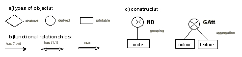
Chapter 2 already discussed the three levels of design of an information system, i.e. conceptual, logical and physical. Since we give preference to already designed DBMS, the physical design is completed and our task is limited to the conceptual and logical design. Chapter 5 has already treated issues related to the conceptual design. Here, the mapping into relational data model will be discussed with respect to the SSM and the selecte object characteristics. To facilitate the procedure a semantic model will be used as an intermediate step (see Chapter 2). Of the semantic data models, e.g. the Entity-relationship data model, the IFO data model or object-oriented data models (see Vossen 1990), the IFO data model suits the implementation strategy of this thesis. On one hand, the concepts presented in Chapter 5 follow the object-oriented approach, on the other hand, the intended database system is an RDBMS. The IFO semantic model uses object-oriented notations to represent objects and their relationships and provides a mechanism to map them into a relational model. Three kinds of object-types (abstract, printable and derived) are distinguished by the model (see Abiteboul and Hull 1987). An abstract type is an object that cannot be shown printed, mapped, etc., e.g. a building, a person, a company. A printable type of object is an object that can be printed, shown, etc. e.g. the address of a person, co-ordinates of a building, a name of a company. The objects that are composed of some printable objects or other atomic objects are derivable. From atomic (printable or derivable) objects complex objects can be derived by aggregation and grouping. The principle difference is that aggregated objects contain elements from different types, while grouped objects contain objects only from one type. IS-A relationships are utilised to define sub-types (specialisation) and super-types (generalisation) of objects. Figure 7-2 shows the graphical notations for the objects, relationships and principles of construction.

Figure 7-2: Notations of IFO data model

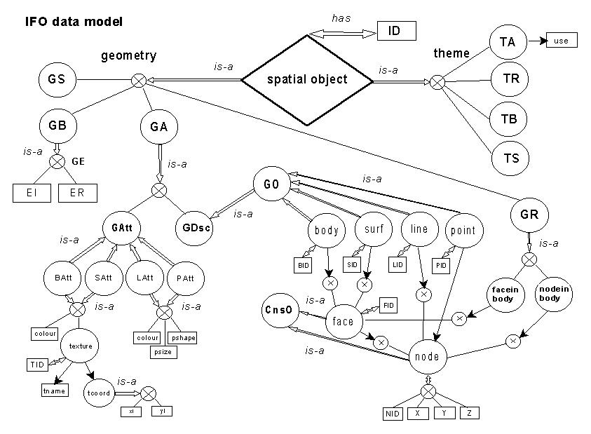
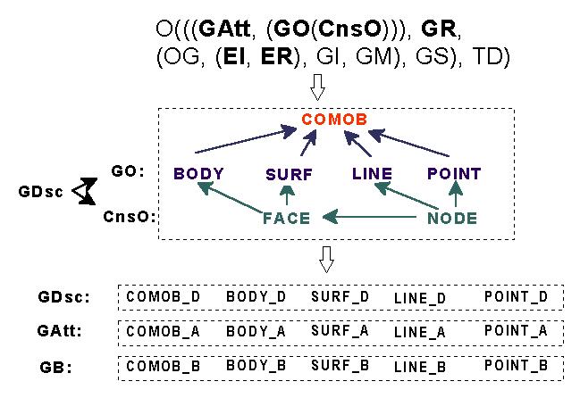
The logical model presented here is not a complete implementation of all the components of the object defined in Chapter 5. We concentrate mainly on GA, GR and GB, assuming that they represent the most important information for creating VRML documents and have a crucial impact on the successful communication between client and server (see Figure 7-4). The geometric description of the objects, however, is complete and corresponds to SSM. Following the principles of the IFO data models, limiting the scope of considered objects to spatial objects and emphasising only the geometric domain (GB, Gatt and GDsc), we arrive with an IFO semantic model, which we will name Simplified Spatial Schema (SSS) (see Figure 7-3)

• abstract object types are represented as relational tables (or relations)
• derived object types are represented as relational tables or domains (if they are atomic objects to a complex object)
• printed object types are represented as domains
• IS-A relation is propagated until a printed object type.

R = ({A₁, …, A_n}, {PK}) where R = () is the relational table, {A₁, …, A_n} are domains and {PK} is the primary key. Then we obtain one mapping into the relational data model (see Table 7-1, variant 1).

The Gatt and GDsc are expressed by one of the tables X_A or X_B, where X may be BODY, SURF, LINE and POINT. Another way to convert the conceptual model into relational tables is the propagation of the ID of GO to the spatial object and utilising the ID of the GO for the identification. This is possible only if the functional relation between GO and GO is 1:1, i.e. a spatial object has only one geometric representation. In this case, the first table is not necessary but separate tables for GB and TD according to the XID have to be created, i.e.

The second set of relational tables (see Table 7-1, variant 2) may have some advantages when the detailed specification of TD and GB is completed. It might appear that there is a dependency between the type of GO chosen for the geometric representation and the thematic attributes. For example, all the private buildings in a town might be described as bodies with the only theme "owner". Automatic procedures for data extraction and reconstruction vary for different abstractions of real objects. Some of them are fully automatic (DTM), others follow complex reconstruction algorithms. The control of the reconstruction (deleting, adding and updating, associating with thematic classes) is relatively simpler in the second set of tables. Besides, the reconstruction procedure used in this thesis is built on 3D FDS, which maintains thematic class per GO. As a consequence of the considerations mentioned, the tests are completed on the second set of relational tables.

The equivalent set of relational tables can be obtained directly from the notations of object components and SSM given in Chapter 5. The rules for mapping are:

SSM:

• A family set is mapped in a relational table. The primary key is the unique index of the family set.
• The domains of a relational table are 1) the indexed sets and 2) the supplementary index.
• The relational table obtained from the family set ND has domains X,Y and Z co-ordinates.
• The relational tables obtained from the family sets NIB and FIB have BID as a domain.

• The brackets () in the notations are 1) aggregation if the components inside are at least two and 2) specialisation if the component is only one.
• Each component is mapped into a relational table if it has sub-components.
• Spatial objects associated with one geometric abstraction have behaviour, geometric attributes and theme comparable to the geometric abstraction.

The R-tree is implemented in supplementary tables in the database. The R-tree leaves and non-leaves tables contain information about MBB (minX, minY, minZ, maxX, maxY and maxZ co-ordinates of a R-tree box) and the identifiers of the three children leaves (non-leaves). The number of entries, i.e. three, was chosen among experimented 2,3,4 and 5 entries per non-leaf. The intention was the preservation of the shape of the grouped objects. An experimented criterion for grouping was the minimal oblique distance, the minimal horizontal distance, and the min-max angle between weight centres of the objects. The best results were achieved with the criterion min distance and min-max angle between mass centres of the objects (see Chapter 8).

On the basis of the R-tree, an indexing schema is introduced. Since the indexing schema is not database-implemented, it will be referred to as a code. The code has variable length depending on the height of the R-tree and different min/max values related to the entries per leaf. For example, an R-tree with height 7 and entrance 3 (the resulting R-tree of the experimental site "Vienna") will have a minimum value 11111111 and a maximum value 3333333. The last figure of the code shows the place of the object on the leaf level. Since the R-tree is created on the basis of MBB of GO, some CnsO might be common for one or more GO. Furthermore, they may continue to be common for bounding boxes. Hence, each GO gets a code according to the place of the objects in the R-tree. The code that CnsO gets has following properties:

• is the same as the GO’s if this is the only occurrence of the CnsO
• has zeros at the positions where the codes of GOs having the same CnsO differ, e.g. if GO₁ has a code 3221123 and GO₂ has a code 3221131, then the common CnsO (e.g. face) will have a code 3221100.

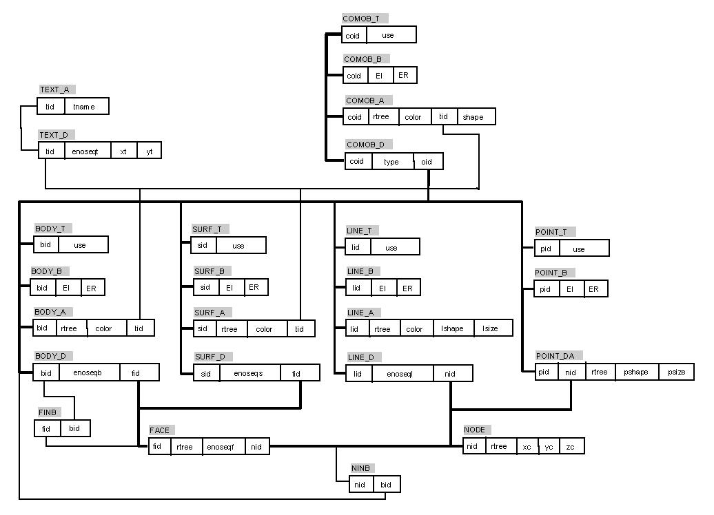
Bearing in mind initial ideas about the composite object (complex of different geometric objects), experimental relational tables were added to the database. The composite object is represented by its composing objects as an indication of their origin, i.e. body, surface, line and point is provided. Since the composite object is a GO, the same four types of relational tables, i.e. _A, _D, _B and _T, are created. The final relational database schema is represented in Figure 7-5. Samples of the relational tables are shown in Appendix 4.

In summary, SSS differs in several aspects from 3D FDS:

• parameters describing the behaviour of objects are introduced
• parameters describing radiometric properties of objects are included
• the information about texture is maintained per object (surface and body)
• the arcs are not maintained
• the geometric object body is explicitly described by faces
• lines and points are represented by nodes and bodies and surfaces are represented by faces
• sequence of the nodes in a line is indicated
• arc-on-face, arc-in-body and node-on-face relations do not exist, but a new relation face-in-body is introduced
• composite objects are introduced.

7.3 SSS and procedures for data collection

Spatial objects (i.e. topographic and fictive objects) of common interest for a municipality include buildings, transportation network (e.g. streets, bridges, railways), sewer and water networks, telecommunication and electricity networks, parcels, other boundaries (e.g. neighbourhoods), vegetation, other man-made objects. In general, current GISs may already contain a sufficient amount of data for a description according to SSS. Depending on the data, different steps to convert them into SSS have to be followed. Objects that are associated with surfaces (e.g. streets, railways, parcels, neighbourhoods, parks, trees) will commonly require a set of operations to be performed: check for the number of nodes, check for face planarity (if the nodes are more than three), check for face orientation, check for existence of holes. Surfaces and lines parts of the terrain, which are available with 2D co-ordinates, first have to be incorporated in the Digital Terrain Model (DTM), often available as a Triangulated Irregular Network (TIN). Since such a procedure will triangulate the surface objects, the control over the number of nodes, planarity and orientation of faces, and existence of holes is not necessary. Surfaces and lines that are not part of the terrain (e.g. fences, elements of bridges and buildings, telecommunication, electricity, water and sewer networks) require supplementary height information. It can be collected either by extra measurements or from existing records, e.g. the depth of the water network. Objects with complex 3D geometry, however, need more sophisticated procedures for 3D reconstruction and recording in SSS. The next two sections discuss this issue in detail.

Data about geometric attributes have to be either adapted from current information systems, or specified in addition. For example, the colour of objects is not of primary interest to 2D users due to default colour palettes provided by the information systems. Therefore, records specifying colour parameters do not exist. The texture widely applied for 3D city modelling is usually "stored" in the drawing files used for visualisation and hence not applicable immediately for the data organisation in SSS. Section 7.3.3 elaborates on texturing procedures.

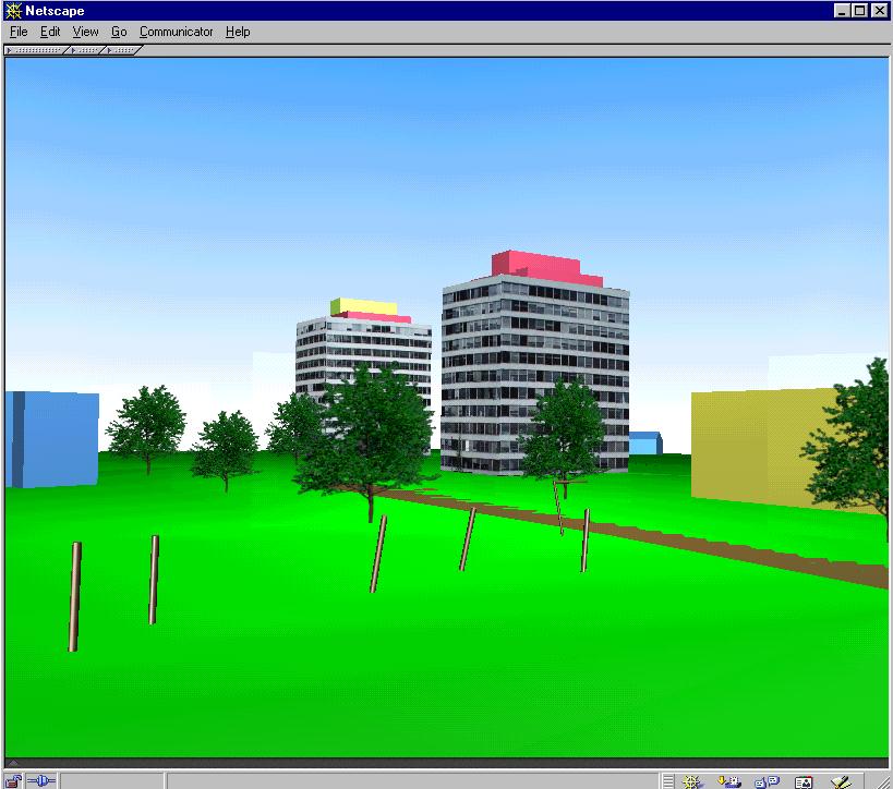
The two fields in the logical model (i.e. lshape and lsize in LINE_A and pshape and psize in POINT_DA) allow predefined primitives (i.e. cone, cylinder, sphere, billboard) and the corresponding parameters to be specified. The parameters can be related to the real size of the objects. For example, the lampposts of Enschede (see Figure 7-7) are visualised as cylinders (in lshape) with a diameter 0.30 m (in lsize). The length of the cylinders is computed on the fly on the basis of the nodes constituting the line. The co-ordinates of the node give the position of the lamps. The trees are visualised by billboards or the 3D symbol of a tree specified in the field shape. The height of the tree is defined in the field size, and the position is obtained from co-ordinates of the point (see Appendix 4). Clearly, first the manner of representation in the virtual world has to be decided and then algorithms have to developed for converting existing data.

Organisation of geometric behaviour requires more effort since separate units (files, programs, scripts) have to be generated. To illustrate the idea, two files are created and stored for a number of objects, i.e. the panorama movie to visualise interior and the script to show the textured facade. The name of the interior file is stored in the ER field and a parameter indicating the on-click event initiator is stored in EI of BODY_B table (see Appendix 4).

7.3.1 GDsc: procedures for semi-automatic 3D object reconstruction

Most of the current research efforts are directed towards automatic methods for the reconstruction of man-made objects. Among them, buildings are the focus of the research. The regular shapes (e.g., rectangular shapes and vertical walls) of some of the buildings often give a misleading impression that reconstruction of the building from its geometric primitives is an easy task. The lack of operational automatic methods for building reconstruction is an indication that the task is not as easy and simple as it seems. In general, two different approaches, i.e., "top-down" and "extrusion", are utilised to reconstruct buildings. In the first approach, the measured elements are upper parts of buildings, e.g., roof outlines, while in the second, the reconstruction starts from the footprints. Which method is better depends upon a number of considerations such as the desired resolution (complex roofs or rectangular boxes), available data sources (2D GIS and/or aerial images), hardware and software, the purpose of the model. The roofs of the houses exhibit a variety of shapes, which make their classification challenging but necessary for the establishment of a standard procedure. The top-down approach allows more details about the roofs to be collected but requires longer and complex processing of data. Current automatic methods require manual work for grouping and cleaning the data set (see Hendrickx and Vandekerckhove 1997, Gülch et al 1999), or for matching and fitting predefined shapes (see Brunn et al 1996, Grün and Wang 1998).

The extrusion method is applicable in the case of known footprints, e.g., from cadastral maps, and heights derived from images without roof detail (see Lammi 1997). Although the resolution of the model is very low, the algorithms for reconstruction are simple and allow fast implementation. For example, the GIS vendor ESRI has already released extensions to available software utilising this approach (see Pilouk et al 1997).

Although advances have been reported in automatic building extraction, human intervention at some stage of the process is still indispensable. The more complex the topography and the higher the required resolution of its model, the superior is human interpretation of the stereo model. It can be coupled then with simultaneous manual digitising. The operator can better judge the composition of a building. Consequently, a sufficient number of optimally distributed points can be measured, which reduces the time and effort in editing. It also offers the possibility to process a greater variety of features than could not otherwise be done.

Considerations that motivated investigations into an approach based on manual digitising and successive automatic reconstruction can be summarised as follows:

• lack of fully automated reconstruction in the near future
• complexity of urban topographic objects and flexibility of the manual process of reconstruction
• 3D topologically structured data facilitating 3D spatial analysis
• feasibility of implementation on commercially available systems
• preservation of the original measurements.

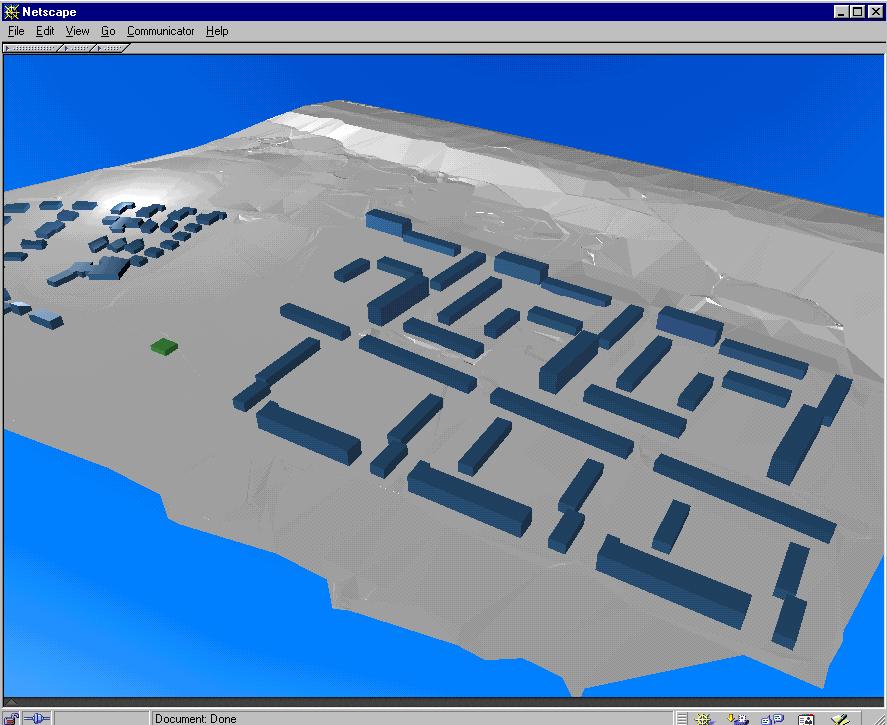
Figure 7-6: Enschede: a layer-oriented model                                                          Figure 7-7: Enschede: an object-oriented model

To overcome some of the problems of the procedure concerning data editing, automatic 3D topology creation and thematic classification of objects (see Tempfli and Pilouk 1996), a new approach was proposed by Paintsil 1997.

The new procedure utilises the same hardware but new software, i.e. Microstation. In addition to buildings, the reconstruction surfaces, line and point objects such as streets, parking lots, power lines, lampposts, manholes, etc. are provided. The new procedure is object-oriented, i.e. the operator deals with one thematically and geometrically specified object from the starting step, i.e. digitising until the last step, i.e. validation and recording in the database. The procedure for buildings is based on manually digitising the corners of roof facets in a photogrammetric stereo model, thus creating a "skeletal point cloud". The reconstruction consists of automatically computing and assembling all the facets of the building from this point cloud. The model obtained in this way contains planar closed polygons (faces) which are oriented to meet the requirements of rendering engines, i.e. the normal vector of the faces points towards the outside of the building. The reconstruction rules for other topographic objects are in most cases simpler than those for buildings.

The process of reconstruction assumes that buildings have only vertical walls, without windows and doors, and non-over-hanging roof facets, i.e., roof outlines are projected to the DTM to obtain their footprints. If specifications ask for differences in projection between roof and building floor, additional measurements and/or computations are be required. Lean-to roofs, not being part of a solid object, are digitised and stored as surfaces. Depending on the terrain, the wall obtained from the procedure may not be strictly rectangular. An idea to have in the model only rectangular faces is discussed in Zlatanova et al 1996a. While appropriate for texture mapping, the approach creates problems in maintenance of 3D topology.

The main steps involved in the procedure are DTM creation, data acquisition, data processing, superimposition, database updating and visualisation in VR browser and Microstation.

A key element in the building reconstruction approach is the DTM of the area. The DTM has to be generated in advance. Various methods such as photogrammetry, surveying, etc., can be applied for this purpose. The experimental work showed that generating DTM automatically is not suitable for densely built-up urban areas. Firstly, editing the automatically generated DTM is time-consuming and creates a large number of terrain points. Secondly, often a lot of features coinciding with the ground surface (e.g. streets) have to be digitised anyway. Moreover, they should be digitised prior to measuring spot heights because they have to be included in the TIN generation. The number of measured points and their distributions in urban areas is usually sufficient for creating TIN. It is later used to reconstruct the buildings For example, the Enschede model is reconstructed on the basis of TIN created by digitising only those points necessary for describing surface objects (see Figure 7-9).

The process of data collection consists of measuring the points of interest from the stereo model in the TRASTER and extracting their co-ordinates into files using an extension of Microstation (MDL application). The only restriction on the sequence of digitising, i.e. anti-clockwise, is imposed in order to facilitate the orientation of faces. The co-ordinates extraction is done by bordering the points constituting a roof facet with a fence (a tool of Microstation) and recording them in a separate file. In this way, all the facets of a particular roof are stored in a set of files. Digitising of other objects of interest is done similarly.

According to the types of object, different parts of in-house developed software are activated. For example, buildings are processed according to the type of roof, as three types are currently supported (see Figure 7-10). The software automatically builds the files as the content corresponds to the logical model of 3D FDS. The files which refer to the explicit relations (arc-on-face, node on face, arc-in-body, node-in-body) are not included, due to the impossibility to collect the information observing the model. Thus the processing leads to the building of 3D topology according to nine tables of 3D FDS. More details about the procedure can be found in Paintsil 1997 and Zlatanova et al 1998.

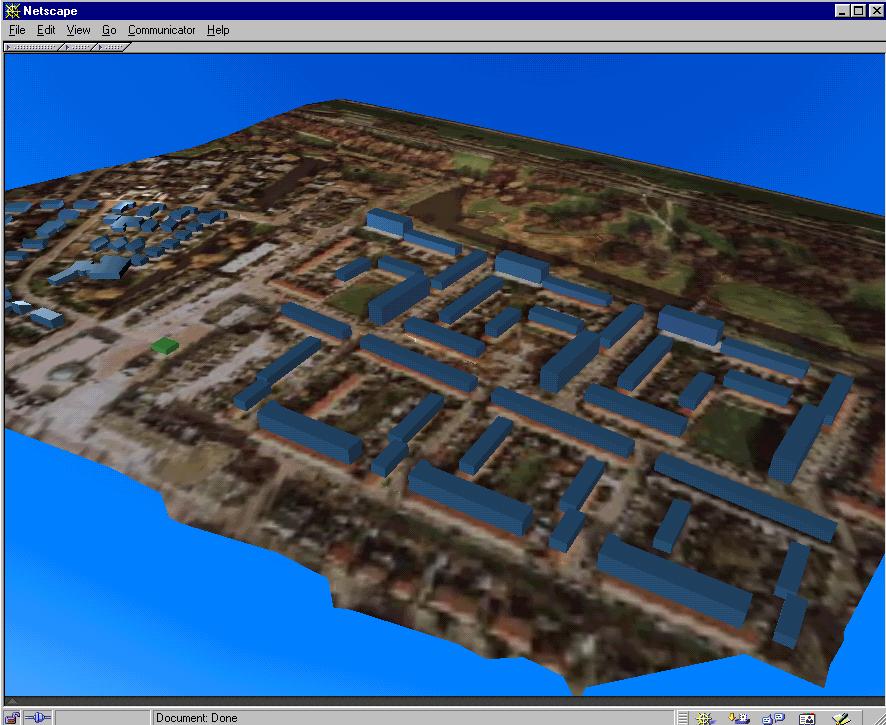The procedures allowed new objects to be added to the model, i.e. lampposts, streets, parking lots, trees (see Figure 7-7) as well as gable roofs to be processed (see Figure 7-13). Compared with the first approach, several advantages and improvements are achieved:

• objects are identified and classified by the operator during the digitising steps
• topological relations are established with respect to already existing objects in the database
• the reconstruction can be verified per object by visual inspection of the object: 1) in a VR browser (for gross errors and correct orientation of faces) and 2) superimposed in TRASTER (for the precision of the digitising and TIN creation)
• the object is recorded in the database only if the operator is satisfied with the results, i.e. the database is not violated in the case of incorrect reconstruction.

In our experience, the main disadvantage of the procedure is the manual grouping of digitised points and extraction in separate files. Therefore, the software for processing was modified in two ways: 1) processing of closed polygons instead of point clouds and 2) extraction of more than one building in a single file. The hardware platform was changed to PC with software packages SOCET SET and Microstation. Indeed, the buildings have to be of one geometric type, belonging to the same thematic class. For example, all the residential buildings with flat roofs can be extracted in a single file. The operator is allowed to decide how to proceed later, i.e. the reconstruction will be performed either at once for all the buildings or one by one followed by visual inspection. The process gains in speed, but a possibility for confusion with already reconstructed buildings exists. The software was tested on a data set (Rozenburg, The Netherlands) obtained from manual digitising for 2D cadastral maps. The roofs of the buildings were digitised to obtain the footprints that allowed a reconstruction according to the procedure described above. The digitised dense net of surface objects permitted creation of TIN to compute footprints, which were later incorporated in the triangulation utilising software described in Gorte 1994. Since the ridge points of the gable roofs were missing, most of the reconstructed buildings have flat roofs (see Figure 7-11 and Figure 7-12). When the ridge participates in the description of the outlines, then the gable roof is constructed successfully (see Figure 7-13 and Figure 7-14). Since the outlines of the roofs were digitised without due care to the orientation of the polygons, the operator had to be examine each building and ensure the correct orientation.

Figure 13: Rozenburg: trees represented by a model of a tree                     Figure 14: Rozenburg: trees represented by billboards draped with an image of a tree
 

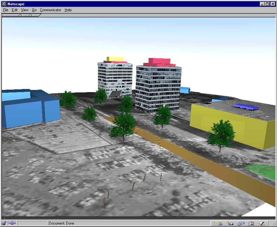
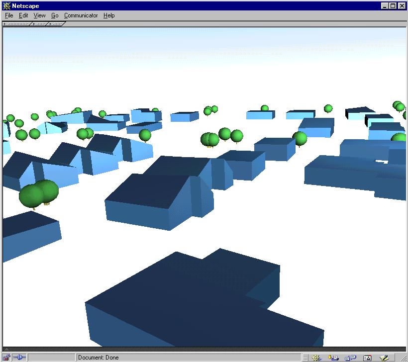
Images mapped on billboards preserve the real appearance of the tree, which might be a consideration for parks with specific and unique vegetation. The VR model, however, is slower for parsing and navigation through. A disappointing (for some users) effect occurs if the model is observed from a bird's view, i.e. the 2D shape of the billboards is visible. The 3D symbols are a better solution in the case of many trees: the VR model reacts faster and the display time is shorter. Figure 7-13 is a snapshot of the same data set where all the trees are represented by a 3D symbol composed of one sphere and one cylinder.

An advantage of 3D symbols is the fewer parameters for storage in comparison with billboards. The symbol tree here is organised as a separate VRML file, whose name is stored in the field shape. The field size provides the size of each particular tree in the scene, according to which the symbol is scaled. The billboard representation requires in addition the organisation of images. The image of the tree used here is adopted from Ames 1996.

Although encouraging results were obtained from the reconstructing experiments, a number of problems require more investigations. One area is extending the procedure and algorithm of reconstruction to cope with occlusions and geometric constraints. Another direction for improvements is toward an optimisation of thematic encoding. A third problem area is reducing manual processing by structural analysis of skeletal point clouds or polygons. Mwewa 1998 reports some initial ideas in this direction. A fourth area is the ability to define individual parts of the building as separate objects. The procedure to this end creates one object (body) of a building, i.e. its roof and walls are united. Besides disturbed display (buildings appear in one colour), it may be a weak point in spatial analysis. For example, the query "what is the area of the walls" needed to estimate the amount of paint for renovation will be difficult to complete.

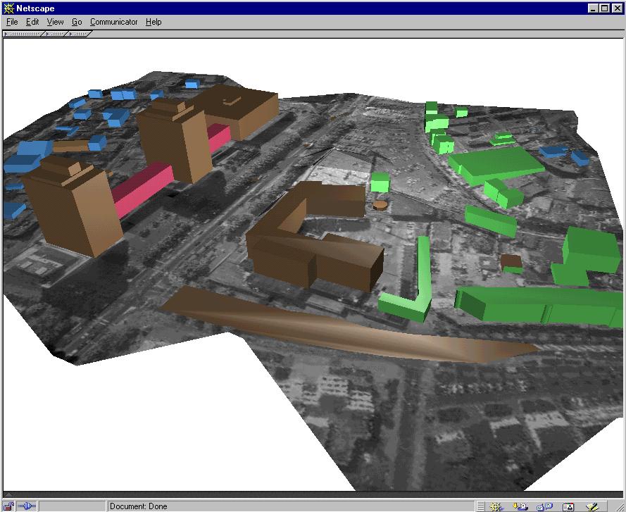
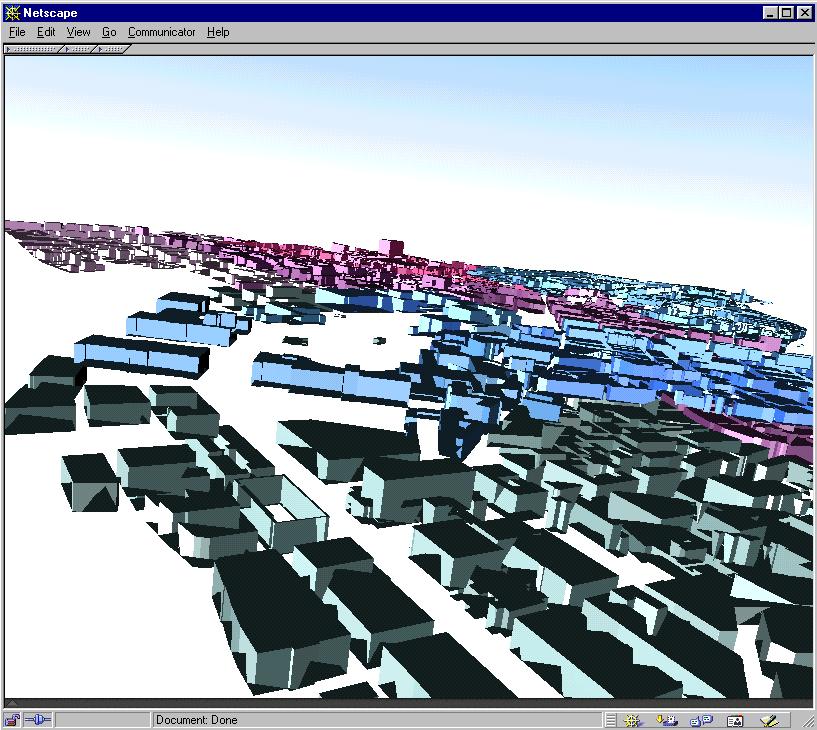
The approach for 3D data collection can be used to supply data for SSS by a conversion of the 3D FDS file organisation obtained from the reconstruction procedure. In-house developed software makes possible the transformation between 3D FDS and SSS. Each object type of 3D FDS is converted to object X_T in SSS. The NODE file is preserved. The remaining files are converted according to the descriptions of the two schemas. The transformation is applied for two test sites, i.e. Enschede and Vienna. The Vienna data set (generated and obtained from ICG, TU, Graz, Austria) is transformed from SSS to 3D FDS (see Figure 7-15). More details about the conversions can be found in Chapter 8.

7.3.3 GAtt: texture and texturing

A common procedure to collect geometric attributes, i.e. colour and texture, was not available. The data collection of these parameters is a mosaic of different approaches, which will be briefly mentioned here. The colour of objects was not of primary interest and therefore it is determined on the basis of the theme of the objects under which they are digitised.

The process of texturing is a broad issue requiring inter-disciplinary research related to image capturing, image processing, image mapping (or draping) and storage of textures. The entire process will be only briefly reviewed, since only the organisation of texture is relevant for this thesis.

The first problematic issue is the automatic collection of images. While appropriate for texturing terrain and roofs, often the aerial images often are not sufficient to texture facades of buildings. The distortion of the facades in nearly vertical images, the image scale, the shadows are some of the disturbing factors. Still, the widely applied method to collect images for texturing of facades is manual. Some advances toward automation of the process are reported by Maresch and Scheiblholfer 1996.

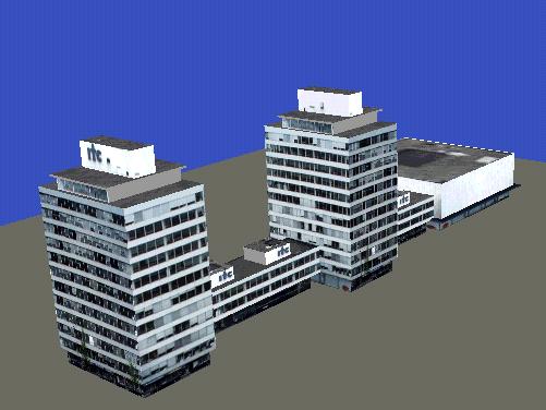
                                         Figure 7-15: Vienna: buildings                        Figure 7-16: Enschede: The old ITC building modelled at ICG, TU, Graz, Austria
 

The collection of images for texturing raises two challenging issues related to image storage, i.e. the resolution and the colour of the images. Usually, the space needed for storage of texture is much larger than the geometric description (see Kofler 1998). This requires a prior decision to be taken on the way of texturing and an estimation of the expected size of the database to be made. For example, the resolution of aerial photo images might not be sufficient for frequent walks through (ground level) the town. The street level of buildings' facades being occupied by shops, offices, etc., may need more detailed images than the second and higher floors, which usually are mostly private apartments (see also Gruber et al 1997). The consideration is the colour of the images. Grey images consume less storage space than colour ones but the information supplement is less (compare Figure 7-9and Figure 7-12). The usage of colour images is influenced by practical factors, such as intended number of textured objects, purpose of texturing, availability of images, hardware and software for processing and visualisation. A variety of combinations are possible: i.e.

• grey aerial photo images to drape the terrain and colour camera images for facades (see Figure 7-7)
• colour aerial images for terrain and non-textured buildings (Figure 7-12)
• colour images to map facades and non-textured terrain (Figure 7-16 and Figure 7-18)
• colour images to texture entire model (see Leberl and Gruber 1996).

The extraction of parts of images is the activity that requires most automation. The need is especially urgent for the process of texture mapping (see Chapter 4). Still, the widely applied method for texture mapping is manually adjusting the image onto geometry in CAD (3D MAX, Wavefront, RenderMAN) and VR modellers (Medit, PioneerPro, CosmoWorlds). Sithole 1997 reports an automatic procedure (and a prototype system) for texture extraction from aerial stereo images with respect to existing geometry provided in a DXF file. With respect to an angle threshold, each face of the geometry is tested as to whether it can obtain a texture from the image. In the case of a positive test, the co-ordinates of the face are mapped onto the image. The pixels of the image corresponding to the area of the face are rectified (and resampled) and converted in a separate JPEG file. The author suggests an extension of 3D FDS to cope with all the possible relations between a face and a texture, i.e. a single texture per face, a multiple texture per face, a single texture per object and a multiple texture per object. Since the procedure establishes a link between co-ordinates of faces and image co-ordinates (i.e. it is a texture mapping procedure), it can be easily adapted to SSS. The texture storage per object (surface or body) provides an implicit link to the face (will be discussed).

7.3.3.1 Texture mapping: buildings

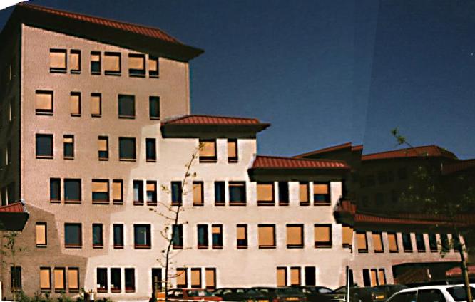
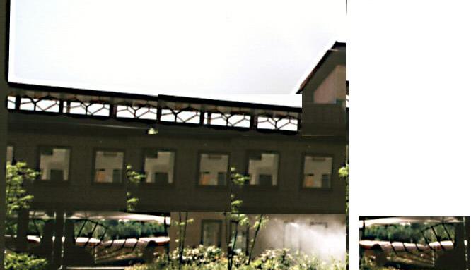
With respect to the fourth objective of the thesis, it was important to experience the methods for texture mapping supported by the current commercial systems and their applicability to texture complex buildings. The ITC building was selected for experiments due to the complex geometric description, the variety of different facades, and a number of problems in obtaining good images. With respect to 3D modelling, the building is an example of the optional higher resolution demanded for some buildings (see Chapter 3). As was mentioned, prior to object reconstruction, it has to be clarified which approach is to be adopted, i.e. a resolution applying detailed geometric description or a resolution applying realistic texturing. The model of the ITC building was already available in a detailed geometric description (walls, windows, complex roof facets), created by Pilouk (see Tempfli and Pilouk 1996) by manual digitising of architectural plans (see Figure 7-17). Here we will concentrate on the collection, processing and mapping of images.

 
Figure 7-17: ITC building (adopted from Tempfli and Pilouk 1996)                         Figure 7-18: ITC building: textured with real photo images
 

Figure 7-19: ITC building: reduced geometric detail	Figure 7-20: ITC building: increased details by texture

The texture co-ordinates and the newly designed faces are imported in SSS by in-house software for a conversion between VRML (supported by Medit) and SSS. The building is a composite object of many surfaces specified as different walls and a roof. The relationship between a surface and a image file is one-to-one. This is to say that an image file that contains texture for a particular surface, obtains a texture identifier (tid). The image co-ordinates are recorded in the table TEXT_D in an order that corresponds to the order of faces (enoseqs, in SURF_D) and the order of nodes (enoseqf, in FACE). The table TEXT_A establishes the link between the texture identifier and the physical name of the image file. Thus, employing the explicit enumeration of faces in a surface and nodes in a face (see Figure 7-5), a simplification of the solutions for database storage proposed by Sithole 1997 is achieved.

7.3.3.2 Texture draping: terrain

The second mechanism for texturing supported by VRML, i.e. texture draping, can be maintained in SSS as well. As already mentioned, texture mapping may appear an accurate mechanism for some objects, e.g. the terrain. Indeed, if the user demands terrain details, e.g. the patterns of the street's coverage, pedestrian areas, gardens, then the overall process of texturing must follow the steps discussed above. In the case of nearly vertical images, the approach of Sithole 1997 can be applied to extract parts of images per terrain face. Similarly to facades, the textures for faces constituting surface objects (on the terrain) have to be organised in one image file.

Since the draping mechanism does not require referencing between image and face co-ordinates, the data storage is simpler: the physical name of the image file has to be specified in the table TEXT_A. The image, however, has to be oriented in a way appropriate for the mechanism adopted by VRML. Recall Chapter 4 and the draping mechanism of VRML. The image is spread over the entire shape according to a rule (see Figure 4-2). When the object is represented as a surface, a MBB is created around the surface, the texture is wrapped onto MBB (according to the rule for a box) and then the image is projected on the original surface. Depending on the surface, this technique leads to different distortions of the image. The parameters to compensate for these distortions are scale (s_x, s_y), shift (x₀,y₀) and rotation (a ), i.e. five parameters. Since SSS does not maintain additional fields for these parameters, the image has to be pre-processed according to default values of VRML. Figure 7-23 shows the steps to achieve an image ready to drape on a surface in VRML, i.e. geo-referencing, re-sampling, determining the area of MBR on the image and clipping off. The procedure, followed in our cases (see Figure 7-12) is:

• image geo-referencing utilising between six and 10 ground control points (in ILWIS)
• image re-sampling (in ILWIS)
• computation of s_x, s_y, x₀, and y₀ to match the image size with the size of the MBB (in-house software).

Figure 7-23: Pre-processing of an aerial image for texture draping

7.4 Summary

The chapter has elaborated on the implementation of the conceptual organisation of thematic and geometric data into a relational database. Among the components of a spatial object, the emphasis was only on geometric description, geometric attributes, geometric behaviour and theme. These components are considered sufficient to build a prototype system and evaluate the rationality and efficiency of the new concepts. The chapter demonstrated that an existing procedure for 3D object-reconstruction can be adapted to provide data for SSS. The established geo-reference between image and face co-ordinates, obtained from manual modelling (in commercial software) and an experimental automatic procedure, can be readily stored according to the texture organisation in SSS.

Realisation of the concepts in the relational database systems has followed the two major stages of database design, i.e. conceptual and logical design. The logical design was completed applying 1) the principles of the IFO model and 2) straightforward mapping from our definitions into relational tables, applying a number of rules. The resulting relational tables from both approaches are identical; that is a positive indication of the efficiency and sufficiency of our formulations. The logical model portraying the objects of interest, their relationships, behaviour and attributes is called the Simplified Spatial Schema. The model consists of 22 relational tables. Compared with the relational implementation of 3D FDS, the number of tables is essentially more, i.e. each geometric object of SSS is represented by four tables (theme, geometric description, geometric attributes and theme). This raises questions about the size of the database. Chapter 8, Case study 3, shows that increase (in comparison with 3D FDS) should not be expected. The enlargement is compensated by the lack of arcs in SSS.

An R-tree coding schema has been introduced to serve tasks, i.e. dynamic organisation of LOD and spatial indexing. The MBB of the geometric objects are the leaves of the R-tree. The root of the R-tree is the MBB of the entire town. On the basis of the path from the root to a leaf, an object obtains a code. The code is recorded in an additional field in the relational table containing geometric attributes. The constrictive objects are coded in a way that allows detecting of constructive objects common for geometric objects. Constructive objects that belong to one geometric object can easily be related to their object containers. Thus the code facilitates spatial analysis in two aspects: 1) a limitation of the searching space and 2) a provision of an explicit link between constructive objects and geometric objects. The MBB of the R-tree are organised as separate relational tables, which are to be used to create dynamically LOD. The idea is discussed in detail in Chapter 8, Case study 2.

Although a large part of the data maintained in current information systems can be transformed in SSS with limited effort, many 3D objects require procedures for 3D reconstruction and building of 3D topology. To investigate the suitability of the model for data collection, different software was developed to ensure an organisation according to SSS. Two of the experimental data sets (Enschede and Rozenburg) were constructed on the basis of an existing semi-automatic procedure for data extraction and automatic construction of 3D FDS. Experimental software for a conversion from 3D FDS to SSS and vice-versa was developed that establishes a link between SSS and the procedure. The procedure for reconstruction can be adapted to create straightforward SSS as well. Since the conversion between the two models is simple and 3D FDS models were needed for the test, the procedure was not modified. The operators for a consistency control in the reconstruction procedure are limited to the check of existing CnsO and GO. In this respect SSS also lacks a consistency control. Operators to detect and resolve the configurations node-on-face, node-on-line (a node appearing between two nodes in a line), node-in-body, line-on-face (a line crossing a face with the link between two nodes), face-on-face (holes) and face-in-body has yet to be developed.

Converters between a number of CAD formats and SSS were built. Applying some of them, a third data set, i.e. the Vienna test site, was organised with respect to SSS and 3D FDS. A converter between VRML and SSS provided a way to use the texture mapping completed in 3D modelling software. Applying the converter, the last test site, i.e. the ITC building, was structured in SSS.

Besides the pursued investigation into the techniques to collect data for SSS, the experiments provided a sufficient number of data sets to test the prototype system and the automatic creation of LOD.