2.1.1 Objects, attributes, relationships, operations
2.1.2 Design phases in modelling
2.1.3 Object-oriented principles
2.1.4 Relational data model

2.2.1 Types of objects
2.2.2 Attributes
2.2.3 Spatial relationships

2.2.3.1 Set theory and topology
2.2.3.2 Detection of spatial relationships

2.2.4 Operations

2.3.1 Scene components

2.3.1.1 Points and "empty" polygons
2.3.1.2 "Filled" polygons

2.3.2 Interaction and manipulation
2.3.3 Levels of Detail

2.4.1 Techniques to access data on the Web
2.4.2 VRML: the Web standard for 3D visualisation

The term model is one of the most frequently used words in many disciplines. Scientists build and prove hypotheses, make predictions, exchange ideas and gain knowledge on the basis of models. The model is extensively used to represent certain phenomena in a way readable for others. Hence, the meaning of the term, as well as the principles on which to build models, have to be understandable for everyone.

Many different models exist about various aspects of the world. One categorisation of models can be made regarding the phenomenon to be described, i.e. real or imaginary. In the first case, some properties of the real object have to be selected (measured, investigated, observed) and utilised to create the model. In the second case, the properties have to be designed (planned, computed, decided) by the user and assembled to form the model. A clear boundary between the two models is sometimes difficult to establish. The deficiency of real measurements might be so high that human design is necessary to represent the phenomenon. In both cases, the process of model production is called modelling.

Another categorisation of models addresses their form, i.e. digital and non-digital (e.g. paper maps). Although sometimes better understood by humans, non-digital models cannot be managed by computers. The benefit of using computers for modelling needs no explanation. Models that are intended to interpret the world in a certain way understandable to the computers are called data models (Vossen 1991). In general, data models are simpler than most of the scientific models.

2.1.1 Objects, attributes, relationships, operations

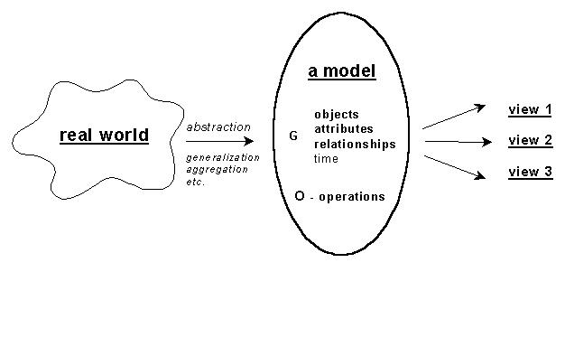
A strict definition of a data model can be found in any book about databases. Here, we adopt the one presented in Tsichritzis and Lochovsky 1982. A data model denoted by M is a tool that provides an interpretation of the world and consist of generating rules denoted by G and operations denoted by O, i.e. M(G,O) (see Figure 2-1). The generating rules reflect two aspects of the model: 1) structure specifications (G_s) and 2) constraint specifications (G_c), i.e. G(G_s, G_c). Structure specifications establish the type and organisation of data, while constraint specifications impose any compulsory model limitations. For example, a real building might be represented in a model as a set of planar, rectangular faces (due to the structure specifications); however, the faces must intersect only along their boundaries (due to constraint specifications). The generating rules operate on data, which are commonly understood as a tuple of objects (categories), their properties and mutual relationships captured in a certain time moment.

Figure 2-1: A model as an abstraction of reality
 

The operations describe all the actions that can be performed on the data as some data models allow standard languages for data manipulation to be established (e.g. SQL). Traditionally, five generic operations are distinguished: set currency (establish a logical position in the model representation), retrieve (make available some data to the user), insert (add new data), delete (remove data from the database) and update (change existing data). Common supporting operations are selection, navigation and specialisation. Selection is an operation that allows a number of data to be identified on the basis of three properties, i.e. logical position (first, last, prior), value of the content or relationship. For example, the user may want to see the first 10 (with respect to the identification number) buildings. Navigation is an operation that permits a logical path on the basis of a selection to be followed. Specialisation is a complex operation that allows a new object (category) to be created on the basis of existing ones. For example, the user may need to provoke the creation of a conglomerate called "shopping centre" of several existing buildings. In some spatial models, the operation will be completed by the Eulers operators for adding and removing elements from a spatial database, in such a way that the structure remains manifold (see Mäntylä 1988). A typical example, which is related to the relational data model, is the creation of a new table on the basis of existing ones. The operation specialisation is then realised by the operations of set theory union, intersection and deletion. Indeed, the user of the model can define as many operations as needed for the specific application.

The possibility for the model to provide users with different, independent subsets of data (called views) is considered an essential characteristic of certain classes of models. More details about views can be found in Vossen 1991.

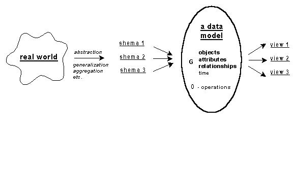
Many models have been developed of varying scope in terms of world representations and generating rules and operations. Some models handle very abstract notions (i.e. database models) and aim at accommodating any type of data; others are more application-oriented and operate with specific types of data (e.g. points, lines, faces in spatial data models). The apparent advantage of the common data models is that the structure and operations are independent of the application and hence the management system built around the model in practice serves any application. The application model is described according to the rules of the common model in a schema (see Figure 2-2). The term mapping is frequently used to describe this process, e.g. "our application model is mapped onto the relational data model". Among the common models only three have become widely used and implemented, i.e. relational, network and hierarchical data models (see Date 1981, Martin 1977, Tsichritzis and Lochovsky 1982). The three models are products of the logical design (see Section 2.1.2) and are sometimes referred to as logical models. Since the relational data model is used later in the thesis, the basis principles of only this model are mentioned here (see Section 2.1.4).

In obtaining a model, three phases can be distinguished: conceptual, logical and physical (see Martin 1977, Tsichritzis and Lochovsky 1982, Vossen 1991). Although the phases refer all kinds of models, the terminology is established by research on models of common purpose. Therefore, exhaustive discussions on the design phases can be found in the literature for database management systems.

Conceptual design clarifies which items have to be included in the model: types of objects, their characteristics and relationships. The resulting product of the conceptual design is a conceptual model or schema. The organisation of all the information that the user wants to store permanently on the disk, i.e. creating views of reality, seems to be a tedious task and requires appropriate abstractions and rules. The research on conceptual (semantic) models, which aims at providing tools to describe real phenomena, is quite extensive and has resulted in a number of more or less sophisticated models. One of the most popular, the Entity-Relationship (ER) model (see Chen 1976) operates with entities, which have attributes and relationships among them. An entity can be anything that has some meaning, e.g. a person, a building, a car, a process. Specific characteristics of entities such as names, colour, address, etc., are referred to as attributes. Since the entities are not isolated in the real world–instead they interact or are associated with each other–the notation about relationship is introduced. The relationship can be one-to-one, one-to-many, many-to-one, many-to-many or IS_A. The last relationship represents specialisation (to be discussed later in the text). These notations and the graphical representation called ER-diagram complete the ER-model. As it can be realised, the model does not support an aggregation mechanism; instead it offers an easy way to derive relational tables for the relational data model. The IFO conceptual model, based on an object oriented-approach and having notations for aggregation, is presented in Chapter 7.

Logical design specifies the elements of the logical model, according to the schema obtained from the first stage. If the data model is a relational data model, the logical design clarifies the tables, columns per table and keys. The identification of the objects has to be ensured by introducing a unique ID. If ordering is needed, e.g. clockwise orientation of faces, it has to be indicated explicitly since the relational model inherits non-ordering properties from sets. Often the logical model is associated with the term data structure, since the structure (i.e. tables, tree or network) of the data is already established.

Physical design is the last phase, establishing the way of communication with the hardware with respect to the logical model, i.e. set of files stored on the disk. The physical design has to enable the operations for manipulating the model.

These three stages of design complete the design phase of the model, which is still not sufficient for a system to become managable. Yet, user interface for the interaction and manipulation of the model has to be provided to enable utilisation by the user.

2.1.3 Object-oriented principles
The modelling process requires many assumptions, classifications, abstractions, selections, generalisations, etc., about real objects and their attributes to be performed. Among the variety of different principles, we concentrate on common object-oriented principles, since they are applied in several parts of the thesis.

The object-oriented approach emerged in early 1970 when the first object programming languages (Simula, Smalltalk) were developed. Since that time, the approach has found applications in different areas of human science. The advantage of the approach is the problem-solving strategy encapsulating information, functions and behaviour per object. Thus any problem to be solved is approached from an object (e.g. person, building, street) perspective rather than from a function ("what kind of functions does the system have to perform") or information ("what kind of information has to be supplied") perspective. The approach is built on a number of principles that provide a mechanism to model real objects in more natural way.

The common methods facilitate the organisation of objects' characteristics and their relationships with other objects.

Objects and attributes: An object can be anything, i.e. person, action, process and the attributes represent all the characteristics. Methods, processes and functions denoting behaviour aim to represent the dynamics of objects. For example, an object can be a building with attributes colour and height. Its behaviour can be the ability to be created, edited, selected, etc.

Wholes and parts: The method has at least three variants: "assembly and parts", "container and contents" and "group and members". The first relation represents the obvious link that exists in manufacturing parts. The door is a part of a car, the window is a part of a wall, etc. The second variant helps in cases when the "things" are not really designed for each other. A typical example is an office, which consists of a desk, a computer, a chair, and bookshelves. The third expression comprises relations that may appear in formations like faculties and courses, groups and subgroups. The members of a subgroup are considered members of the group as well. For example, the group of ITC students consists of the students of courses GFM, GIC, GIR, etc. The principle behind the whole-part method is aggregation. Each whole aggregates a given number of parts, i.e. the cardinality (object connection constraint) of relationships has to be indicated. The relationship is usually read from top to bottom, i.e. consist of.

Classes and instances: Each object has to be organised in a class as the classes are formed with respect to common attributes and behaviour. Each object of a class is an instance of that class. For example, the ITC building is an instance of class Buildings in Enschede. The mechanism to form classes or specify new objects is known as generalisation-specialisation. The generalisation part is applied when a class has to build, i.e. the new class "accepts" (some of) common characteristics of objects and thus creates a more general view about a certain group of objects. The new class becomes their parent and the objects are its children. The children inherit the common properties from the class and contain only the ones specific to them. The specialisation part of the mechanism is used to create children. The number of classes and, respectively, children is not limited. Thus a hierarchy is built as the generalisation mechanism extends the hierarchy upwards and the specialisation mechanism downwards. In through contrast to wholes-parts, the classes-instances relation is read from bottom to top, i.e. is a.

Abstraction is a principle considering the characteristics of an object that are important for the problem or application. Some details quite important for one application might be irrelevant for other. Abstraction is the first principle, which has to be thought for object identification. The characteristics of the objects can be clarified only after an accepted level of abstraction.

Encapsulation is an object-oriented programming mechanism to combine an object characteristic and a corresponding behaviour. Furthermore, the particular software design unit (subroutine, method) could be hidden from the user. For example, a "click" with the mouse on a building (on a monitor) may visualise the owner of the building. The event "click" detected by the system activates the retrieval of a particular object’s characteristic. In this example, the user action "OnClick" and the operation "retrieve owner" are encapsulated in one single method (behaviour). The encapsulation principle applied to the organisation of data can be understood as providing (or not) access to parts of the data and operations. Certain responsibilities can be assigned to parts of the information to restrict operations on data. For example, a common user of a municipality GIS may not be aware of actual geometric representation of a building and consequently not allowed to change the geometry.

Inheritance is the mechanism to express similarities (common characteristics) between objects. As mentioned above, it is the basic mechanism for building classes and thus helps in propagating properties from parent to child. In general, all the attributes and behaviour of a parent are inherited by the children and grandchildren and so forth. The overriding and expending of parent attributes and behaviours is allowed as well. The case where a child has only one parent is known as single inheritance, while multiple parents invoke multiple inheritance. These supplementary techniques are useful for creating composite classes. Opponents of overriding and extending, and multiple inheritance say that the simplicity of the model is lost and that operation with overridden attributes is more complicated. An alternative is introduction of local and inherited properties.

Polymorphism is the ability of objects to have different forms. For example, an object changing its geometry from very detailed to a simple cube is a morphing object. A bank transfer may settle a tax payment by filling out a form or by e-mail. All the operations are valid, therefore the tax payment is considered polymorphic. Polymorphism is a widely used mechanism to speed up real-time navigation inside 3D models. Each object or groups of objects have several geometric representations and the visualisation software decides which of them has to be used. Attributes of objects can be polymorphic as well. For example, an attribute document number can be associated with a parcel as a property document and a person as a document for ownership.

Association is a mechanism to establish a connection between the objects in two classes. The relationship is not typical for the entire class and in this sense can not be resolved by aggregation. For example, class Building and Street can have a connection concerning the relation "building on a street". This leads to the construction of a new class Building-on-Street. Either of the two classes Building and Street is a part of the new class, therefore no aggregation can be applied. However, the cardinality must be known. The similarity between the aggregation and association mechanisms is quite high and sometimes it is hard to decide which mechanism to apply. The basic rule is that aggregation is a class connection pattern, while association is object connection one. Several associations have become well known and used, and have their own name, i.e. participant-transaction, place-transaction, participant-place, transaction-transaction, peer-peer (object connection between objects in he same class).

2.1.4 Relational data model

The relational data model based on relations and their representation as tables was introduced first by Codd (see Codd 1970). The basic category relation is defined as follows: R is a relation on given sets D₁, D₂,…,D_n if it is a set of n-tuples, each of which has its first element from D₁, second element from D₂ and so on. The sets D₁, D₂,…,D_n are called the domains of R. The number of the domains is the degree of the relation and the number of the tuples in R is its cardinality. A table represents each relation, and each column of a table is called attribute. One or more relations, then, can define an object type. Thus the database is specified by a relational schema, which consists of one or more relations R. Since the relational schema consists of separate tables, the relationships between the tables are established by a propagation of keys. The key can be composed by one or more attributes. Two constraints must be satisfied: the key must be unique and the key must be minimal. For example, the identification number (ID) of a building can be used as a key. Since representation by tables may easily lead to repetition of information, the optimisation of the model is critical. Normalisation is a procedure to eliminate different types of dependencies among the relations and attributes. Theoretically, five normal forms are defined, however, three of them are commonly considered sufficient (see Smith 1985). The basic concept that the relational data model misses is the existence of constraints on and among the relations. For example, it is impossible to specify that certain types of buildings (e.g. residential) cannot be higher than four floors.

Among the many different languages for data definition and the manipulation of relational data models, the Structured Query Language (SQL) enjoys the greatest popularity. SQL is an English-keyword set-oriented language. The basic concept is that each operation is mapped onto the relation. The effect is similar to scanning the columns of a table and checking for a value or a set of values. For example, for the operation retrieval, all the rows of the table are scanned and the ones where the sought value is found are returned as results. The fundamental set of key words SELECT–FROM–WHERE allows a large number of mappings to be performed. Furthermore, several mappings can be combined to ensure the basic set operations union, intersection and difference. Attempts to extend SQL toward an ad hoc language for a GIS have been made without a significant success. Egenhofer 1992 argues that SQL cannot become a GIS language due to a number of impossible operations: identity queries, metadata queries, knowledge queries (explaining the reasoning), qualitative queries (e.g. which road is wider), display of query (the result is always a new table), modifying the database content from the graphics and modifying the graphical presentation. The inadequacy of SQL is currently overcome by utilising embedded SQL queries. The outcomes of SQL queries are further processed by operators written in standard programming languages (C, Pascal, Perl) called host languages.

Despite all the deficiencies of the relational data model and thanks to the simple concepts and the standard query language, many commercial Database Management Systems (DBMS) have adopted the model that contributed to its successful integration in commercial and administrative applications.

2.2 GIS models

Geo-science specialists are busy with the modelling of real phenomena. A universal model to comprise all the aspects of reality is not practically realisable due to the high complexity of the real world. Different disciplines emphasise different aspects and only these aspects are included in the model. Thus a model considered good for the description of particular phenomena might be hardly appropriate for anothers. Different aspects and characteristics of real objects have led to the existence of several variations in object definition.

The term GIS model is utilised here to denote a data model of the real world. Being a data model for representing real-world objects, the GIS models have the components defined above, i.e. object types, relationships and attributes with corresponding generation rules, constraints and operations defined with them. A GIS model with the corresponding user interface constitutes a 3D GIS. Often the GIS content is specified as data about geometric (shape, size, location) and semantic characteristics (called attributes), spatial relationships and time (see Aronoff 1995, Maguire et al 1991, Molenaar 1998). The functionality of GIS is then said to be the possibility to perform operations on data in order to analyse them.

The following sections present the necessary fundamental concepts related to the representation of objects, attributes and relationships in a GIS context.

2.2.1 Types of objects

Since the interest in geo-sciences has traditionally been directed toward real objects with spatial extent, the differentiation between spatial and non-spatial objects is widely accepted. A spatial object stands for a real object having geometric and thematic (semantic) characteristics (see Aronoff 1995, Maguire 1991, Molenaar 1989, Pilouk 1996). Tempfli 1998c draws attention to a third group, i.e. radiometric characteristics of spatial objects. Current GIS models maintain only spatial objects. Non-spatial objects (organisations, departments, people, goods, etc.) either are the concern of Database Management Systems (DBMS) or are integrated in GIS as semantic characteristics of spatial objects (see Chapter 3). For example, the person, who owns a building (spatial) exists in a GIS as a semantic characteristics "owner" of the building. As will be discussed in this thesis, dealing with only non-spatial objects may be a drawback for some applications.

A further distinction is made between real objects with respect to distinctness of properties, i.e. objects with well defined spatial extent and properties and objects with unknown or non-well defined spatial extent and properties, i.e. objects with discernible (determined) and indiscernible (undetermined) boundaries (see Cheng 1999, Molenaar 1994, Raper 1998). Usually, quite independent research is conducted in both areas. This may cause problems in the case of analysis where objects from the two groups are needed. Pilouk 1996 discusses the subject in details and advocates an integrated approach while modelling spatial objects.

Many real objects need the monitoring of some of their characteristics with respect to time. For example, growth of population may cause the fast conversion of land from rural to urban use, which can have an impact on the entire urban development. The geo-science specialist might need to store and analyse the changes in order to be able to predict and control the process. Similar problems have created the branch of temporal definitions of an object, according to which objects are subdivided into spatio-temporal and non-spatio-temporal (see Pequet 1995, Worboys 1992). Raza et al 1998 present spatio-temporal-attribute objects (STAO) with three fundamental components, i.e. location (spatial), attribute (aspatial) and time (temporal). Cheng 1999 defines a real object by its three aspects geometry, theme and time.

More general definitions of real objects, regardless of the nature of the objects can be found in the object-oriented literature (see Coad and Yourdon 1991, Hudhes 1992, Norman 1996). Coad and Yourdon 1991 denote as an object every item of interest (real object, feature, process) and present a framework to investigate and classify the characteristics of the different objects. Since this framework is used as a starting point for the object definition introduced in this thesis, more details are presented in Chapter 5.

2.2.2 Attributes

The description of geometric characteristics requires a priori clarification of the abstraction of space, the dimension of space and objects, and the method for representation. Conventionally, two approaches to space abstraction are utilised in modelling processes, i.e. field-oriented and object-oriented (see Worboys 1995). The field-oriented approach assumes complete subdivision of the space into smaller, regular partitions, e.g. pixel. In the object-oriented, the space is "empty" and all the objects are places (embedded) in it, i.e. a lake in a 2D map. Both approaches have advantages and disadvantages and are appropriate for different applications. While the field-oriented approach better suits the representation of continuous phenomena, e.g. height fields, rainfalls, the object-oriented approach represents better discrete phenomena, e.g. buildings, roads.

The dimension of space is defined in mathematics as the number n of a sequence of n -real numbers (a₁, a₂,…,a_n), called an ordered n-tuple. All the ordered tuples are called n-space and are denoted by Rⁿ (see Anton 1994). The basic idea is using a tuple of points to define a position in the space, e.g. a pair of points (x and y co-ordinates in Euclidean space) define a position in a plane, i.e. 2D space. The real world is usually represented as a 2D or 3D space. Within the space, the objects have their own dimensionality, i.e. they can be represented by one of the following generic types: 0D (points), 1D (lines), 2D (surfaces) and 3D (bodies) objects. The decision as to the representation of real objects (i.e. point, line, surface or body), is highly influenced by the purpose of the model.

The possible geometric representations are split into three large groups: i.e. raster, vector and constructive primitives. The "building blocks"(named constructive objects in this thesis) in the raster method are regular cells, e.g. pixels (in 2D space), voxels (in 3D space), which fill in the entire object. The representation is simple and easy to maintain, but produces a lot of data for storage, and the overall precision is low (see Aronof 1995). The vector method is based on irregular n-cells, where n={1,2,3} composed of points with co-ordinates. In contrast to the raster method, the cells represent the boundaries of the objects. The last representation, known as Constructive Solid Geometry (CSG), uses irregular 3-cells. An object is represented by a CSG-tree, which holds information about the CSG primitives and the operations "gluing" them (i.e. Boolean operations). The approach is widely implemented in the manufacturing industry. In general, the irregular cells describing the boundaries of the objects allow more precise descriptions of shapes and spatial relationships compared to the raster cells and CSG primitives. Moreover, the visualisation algorithms operate with the boundaries of objects, i.e. CSG and raster representations have to be further processed to determine the boundary. Therefore many applications give preference to the vector approach of description. This thesis is based on a vector representation too.

The vector representations are often referred to as boundary representations (B-rep) or surface representations (see Mäntylä 1988, Worboys 1995). A large number of spatial models are developed and implemented in GIS, CG and CAD systems based on irregular multidimensional cells. The names and construction rules of the cells in the different models usually vary. The simplest set of cells is the set of simplexes, i.e. 0-simplex (node), 1-simplex (arc), 2-simplex (triangle) and 3-simplex (tetrahedron). Composing simplexes, one can obtain more complex objects, i.e. simplicial complexes (see Egenhofer 1989, Moise 1977, Pilouk 1996). Most of the models allow 1,2,3-cells with an arbitrary shape that imposes some supplementary constraints, e.g. planarity of faces, convex shape. The names vertex (point), edge, face (polygon) and solid (polyhedron) are then used in the literature to denote 0,1,2,3-cell. Further details and a discussion on vector models and cell utilisation in 3D GIS are provided in Chapter 5.

2.2.3 Spatial relationships

Three different approaches to encoding spatial relationships are discussed in the literature, i.e. metric, topology and order. The metric is a pure computational approach, based on the comparison of numerical values related to the location of the objects in the space (i.e. the Euclidean space). For example, the spatial relationship between a house and a parcel (e.g. inside, outside, to the south) can be clarified by a metric operation point-in-polygon performed for each point constituting the footprint of the building. Since the metric is built on the notion of the distance function (see the next section), which is dependent on the internal (finite) representation of numbers in the computers, the approach is computational expensive.

The order establishes a preference based on the mathematical relation "<" (strict order) or "£ " (partial order), which allows an organisation of objects similar to a tree. For example, if a building is inside a parcel, the spatial relationship is represented as "building < parcel". The applicability to representing spatial relationships is investigated by Kainz 1989 who argues that it has advantages in expressions of inside/outside relationships.

Topology allows the encoding of spatial relationships based on the neighbourhoods of objects regardless of the distance between them. The main property of topology, i.e. the invariance under topological transformations (i.e. rotation, scaling and translation) makes it appropriate for computer maintenance of spatial relationships. The following section discusses some basic topological issues that the thesis utilises.

2.2.3.1 Set theory and topology

• rubber sheet geometry
• a study of boundaries
• an abstract study of open and closed sets

Topology has been introduced as a discipline of mathematics and the foundations are set theory and metric spaces. Prior to the mathematical definition of topology, we will introduce some basic notations from set theory and linear algebra.

Set: A set is an aggregate of things, e.g. numbers, people, buildings, points. The things are elements of the set.

Indexed sets: Consider sets and the set , where to each element  corresponds a set A_I,, then I is called index and the sets are called indexed sets. Moreover such an indexed family of sets can be denoted by .

Function: A function (or map) f from set A to set B, written , is a subset of with the properties:

• for each , there is some such that , written also as 
• if and , then .

Ifandthen each function

has corresponding induced functions (on sets) and  (usually the same notation of functions is used for elements and sets). In general, when the function (on elements) is performed, then induced function  is true but is not necessarily true. When is true, then f is onto B. One-one is the function , which obeys the rule: .

Relation: A relation R on a set A is any subset of . Thus every function from A to A is a relation but not all relations have the properties of functions. If R is a relation on A and  then the relationship between the two elements is denoted by .

Historically, topology was introduced as an alternative to represent continuity of a space more general than the Euclidean space. The Euclidean n-space is defined as an n-space with operations of addition, scalar multiplication and Euclidean inner product (for complete definition see Anton 1994). On the basis of the inner product, a metric can be defined, e.g. length, distance, angle. The Euclidean space is used as a fundament by Frechet (in 1906) to introduce a metric space, denoted by , whereis the distance function. If is a metric space for each the following is true:

• 
• 
• , if then 
• 

The function is called the metric on M. Inside the metric space the open sets are defined to be:

A set E in a metric space is open iff (if and only if) for each there is an e-disk about x contained in E. The e-disk about x is also defined on the metric space for to be:

.

The e-disks and open sets can be used to define continuity of metric space without referring to the distance. Topology is the next step to deal with continuity without mentioning the distance (see Hausdorff 1914). Topology is derived from the metric space by using the open sets. The definition of a topology is then given as (see Willard 1970):

A topology on a set X is a collection tof subsets of X called the open sets, satisfying:
any union of elements of t belong to t

• any finite intersection of elements of tbelongs to t
• the empty set and X belong to t .

Inside a topological space, the topological primitives, i.e. closure, interior and boundary of a set can be defined. If X is a topological space and , then:

• closure is the set is closed and 
• interior is the set  is open and 
• boundary is the set 

Closure, interior and boundary of a set have a number of important properties (the proof can be found in Willard 1970) i.e.:

• 
• 
• is closed in X iff 
• is open in X iff 
• 
• 
• 
• 
• 

If X is a topological space and , a neighbourhood of x is a set U, which contains an open set containing x, i.e. , where is the interior of U. Chapter 5 utilises the properties to derive the topological primitives for geometric and constructive objects.

Three more definitions that will be used in this thesis are listed below, i.e.:

Connected space: A set X is disconnected iff there are disjoint non-empty open sets H and K in X such that Then X is disconnected by H and K. If no such disconnection exists, X is connected. For example the Euclidean space IR ⁿ is a connected space. Connectivity is an important property of topological primitives and hence plays an important role in derivation of spatial relationships between objects (see Chapter 6 for more details).

Homeomorphism: If X and Y are topological spaces, a function f from X to Y is a homeomorphism iff f is one-one, onto and continuous and f^-1 is also continuous. In this case X and Y are homeomorphic. The homeomorphism ensures the invariance under transformations.

Embedded spaces: If f is everything but onto, then it is the embedding of X into Y, i.e. the expression is "X is embedded in Y by f". The concept of embedding is very important in the modelling process. In fact, if the objects are defined in a topological space (and hence their spatial relationships), they can be embedded in another space without worry about the spatial relationships.

The practical importance of topology for the modelling of the real world is twofold: 1) it provides a formalism to define spatial relationships, and 2) it allows a formal geometric description of objects. The notions of neighbourhood, interior, boundary and closure contribute to: 1) the definition of the topological primitives of objects, and 2) the encoding in topological relationships, i.e. the interrelations between the topological primitives of two or more objects in their neighbourhoods define the topological relationships among objects. For example, if the neighbourhood of a point is completely inside the interior of an object, then the point is in inside the object; however, if the neighbourhood is partially in the object's interior, then the point is on the boundary of the object. Applied to all the points of two objects, this mechanism supplies information on the interrelation of two objects.

The topology can be applied to strictly define the subdivision of the space and derive the shape of objects out of it. For this purpose, an n-dimensional space (Hausdorff space) called n-manifold, in which the neighbourhood at every point is equivalent to an n-dimensional ball, is introduced. Then a subdivided manifold is defined as a pair (M,C), where the M is manifold and C is a complex of cells. Each subdivided manifold has the following properties (see Brisson 1990):

• each (n-1)-dimensional cell is shared by exactly two n-dimensional cells
• given two n-dimensional cells s_i and s_j , there exists a sequence of cells s_i=s_h=…=s_k= s_j such that s_{hÇs k} is an (n-1)-dimensional face
• given any (n-2)-dimensional cell, the n- and (n-1)-cells adjacent to it can be arranged in a single connected alternating cycle.

2.2.3.2 Detection of spatial relationships

A slightly different approach is followed by Clementi et al 1993. Again, the three topological primitives are used but first the type of intersection is clarified and then a detailed evaluation of all the cells composing an object is performed. The approach claims a detection of a larger number of relations, however, at a high computational price.

2.2.4 Operations

Goodchild 1987 specifies the spatial operations, which have to be performed in six groups:

• operations requiring access to semantic properties of one type of object, e.g. houses that belong to one owner
• operations requiring access to both semantic and location information, e.g. houses higher than three floors located to the north of the station
• operations which create object-pairs from one or more types of objects, e.g. all the buildings included in a given parcel
• operations which analyse semantics of object-pairs, e.g. the buildings in a given parcel that have one owner
• operations which require access to semantic and location information for more than one type of objects or object-pairs: spatial interaction modelling requires access to origin and destination of objects, as well as, their attributes.
• operations which create a new type of object from existing objects, e.g. Thiessen polygons or buffering polygons around lines.

• retrieval operations, e.g. what is the current information about a particular building
• query operations, i.e. retrieval under a condition e.g. the houses cheaper than $50 000
• modelling operations, e.g. what will be the state of the data after ten years or the next year (predicting new information).

• retrieval and query of the spatial data, i.e. transformation (geometric, format, geographical, conflation), and editing (edge matching)
• retrieval and query of the semantic data
• integrated analysis of spatial and semantic data, i.e. retrieval, classification, measurement, overlay operations
• neighbourhood operations (search, topographic operations, Thiessen polygons, interpolation, contour generation)
• connectivity operations (contiguity measurements, buffering, network, spread, seek, inter-visibility, illumination, perspective view)
• output formatting (map annotation, text labels, texture pattern and line style, graphic symbols).

• metric operations, i.e. distance, volume, area and length, are selection operations based on shape and size of objects and further processing
• position operations are selection operations based on location (no further processing)
• proximity operations are selection operations based on geometric characteristics and the creation of new object (i.e. buffer)
• relationship operations are selection operations based on spatial relationships (no further processing)
• visibility operations are a selection based on geometric characteristics and further processing
• semantic operations are selections based on semantic characteristics
• mixed operations, i.e. selections on the basis of geometric and semantic characteristics.

2.3 3D visualisation and interaction

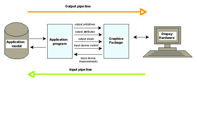
The process of visualisation and interaction is completed in two steps, which are known as pipelines, i.e. input and output (see Figure 2-3). The output pipeline comprises the process of sending information (primitives and attributes) to the screen; the input pipeline comprises the detection of user actions and the corresponding post-processing of the model. The visualisation schema is common for any program, with a graphics output, i.e. CAD systems, e.g. AutoCAD, Intergraph, Microstation, GIS programs, e.g. ArcVIEW, MapInfo, Web browsers, e.g. Netscape, Mosaic.

The application program is the software controlling and ensuring the correct flow of data in both directions, i.e. 1) it accesses the data organised in a model, extracts a subset of data, which has to be on the screen at one particular moment and applying an appropriate graphics package (rendering engine), performs the necessary algorithms to transform 3D graphics to 2D image on the screen, and 2) it controls the input devices. The process of creating images from the model is often referred to as rendering.

The graphics package is a software interface to the graphics hardware, which provides means for the rendering, maintaining windows and detecting user actions. The tendency over the last few years to develop hardware-independent software has resulted in a rendering package, i.e. OpenGL (see Woo et al 1997). From a programming point of view, OpenGL is a set of standard procedures (written in C++) that facilitates the management of graphics hardware. To be able to run on different platforms, the OpenGL syntax does not support procedures dealing with windows and input devices. An application program using OpenGL has to utilise the windowing mechanism and the device tracking (e.g. detecting mouse click) of the current operation system (e.g. Windows, Unix), i.e. make use of corresponding libraries (e.g. Motif X for Unix). In return, OpenGL provides the means: to describe objects, arrange them in three-dimensional space, calculate the colour and illumination parameters and convert the mathematical description of the model to the pixel parameters on the screen. Similar rendering packages, but being less hardware independent, are Direct 3D (Microsoft) and Java 3D (Sun Microsystems), which is the newest 3D interface currently available for two operation systems, i.e. Windows and Solaris.

The visualisation of 3D graphics differs significantly from 2D graphics on several points: 1) scene creation, 2) tools for interaction and manipulation and 3) amount of data. The following text is meant to provide basic knowledge about the mechanisms to obtain readable scenes and ensure sufficient interaction tools.

2.3.1 Scene components

2.3.1.1 Points and "empty" polygons

a)

b)

2.3.1.2 "Filled" polygons

The shading model depends on the method of computing the pixel value across the surface. Several approaches are known: 1) constant shading, called flat or facet – one value is computed and applied to the whole face; and 2) interpolated shading: Gouraund– computation of intensity in every vertex and applying an interpolation across the surface, Phong – interpolation of the normals to surfaces, as the first step is computation of the normals to the edges of the surface.

Complex illumination and shading models to render filled polygons may produce highly realistic scenes. However, they slow down the rendering process tremendously, e.g. applying radiosity (a comprehensive shading technique), a scene might take hours to be computed. Some advantages might be found in the little disk space and memory required to process data. In practice, such models are not relevant for real-world models. Shorter time for rendering can be achieved by utilisation of simple illumination and shading models (i.e. Gouraund and Phong) or texturing. Simple algorithms for shading, however, may create the opposite to a realistic scene. For example, some disturbing effects may occur, like a polygonal silhouette on the edge between two surfaces (see Figure 7-15) or non-constant shading of the surfaces (during navigation through the model). It seems that texturing is the most successful technique to obtain realism in a short rendering time.

Texturing is a technique to wrap an image (scanned real photos or synthetic images) onto the "geometry". The principle is such that, instead of the value calculated from illumination and shading models, a corresponding pixel value (or weighted mean value) from the image (texel) is assigned to the screen pixel. Since the screen pixel value pre-computation is not performed, the rendering is faster. The rendering engine, in this case, must cope with the organisation of images in the memory, as well as, the extraction of each new image needed for a particular scene from the database (see Kofler 1998).

Computer graphics standards (e.g. OpenGL, VRML, Java 3D) give preference to simple illumination and shading models combined with methods for texturing. Thus both rapidly rendered and realistic scenes are ensured at the price of additional maintenance of photo images. For example, the virtual reality browsers are expected to provide only Goraund and Phong models and support texturing (see Chapter 4 for more details).

2.3.2 Interaction and manipulation

The time needed for a system to respond to a user action is the most critical factor in distinguishing between high or low levels of interaction and manipulation. The time interval gives users the perception of being "inside the model", which Isdale 1998 uses to distinguish between off-line plotting, interactive plotting, animation and virtual reality. Off-line plotting is a class of interaction where the user cannot interfere with the process of drawing (e.g. plotting). Interactive plotting refers to systems with tools for interaction and manipulation, which, however, need time to re-compute and render the new scene (e.g. most of the CAD systems). Animation allows the user to calculate dynamics in advance and play it in real time (e.g. 3DStudio, TrueSpace, Wavefront etc.). Depending on animated properties, four types of animation can be defined, i.e. frame, skeleton, morph and interpolation. Frame animation gives the ability to plan the route and the position of the camera, and a sequence of scenes (number of frames is defined by the user) is created. Skeleton animation changes the positions of some geometric elements of the object, e.g. an arm of a body. Morph animation refers to changes in the shape of the object. Interpolation means sophisticated computations between two different positions of an object (see Wavefront 1995). All the types of animation can be observed but not influenced while they are played.

Virtual reality (VR) is the highest level of interaction and manipulation, permitting operations to be completed in near real time. This means that the user does not notice the intermediate calculations between two different scenes. The manipulation and interaction comprise all facilities (hardware and software) that supply users with tools for contact with the objects and directly manipulate them. The perception of the user of interactivity depends to a great extent on the available hardware. While an equipment based on a conventional mouse and 2D screen facilitates only navigation, Head Mounted Display (HMD) (a device which allows displays to be mounted in front of every eye) creates true 3D perception. With respect to the hardware available, VR systems can be classified at five levels:

• Entry VR systems consist of a personal computer (or workstation) with a 2D input device, 2D screen and video accelerator cards.
• Basic VR systems consist of special hardware devices for selection such as PowerGlove, 3D or 6D mouse or joystick, and some enlargement of the display facilities, e.g. stereo graphic viewer.
• Advanced VR systems already include all types of rendering accelerators, e.g. texture, video and powerful processors.
• Immersive VR systems include complex devices for display and sensing, e.g. HMD, CAVE.
• Cockpit Simulators (Cabs) allow physical movements and create a feeling of real participation in the scene and actions.

2.3.3 Levels of Detail

Most of the algorithms developed assume that the LOD are pre-computed different representations of objects. For example, a building may have four different geometric descriptions: 1) walls, roof facets, windows and doors (i.e. LOD0), 2) walls and roof facets (i.e. LOD1) and 3) the bounding box (LOD2) and 4) a single point, e.g. the mass point (i.e. LOD3). All four levels have to be computed in advance and available to the system. Research is conducted toward automatic generation of LOD on the basis of previous scenes, which so far gives good results only for scenes similar to each other (see Aliada 1996). Originally proposed for geometry simplification, the idea of LOD might be extended to the images used for texturing (see Maciel and Shirley 1995). The principle is the same: an image used for a closer object has a higher resolution than the image applied for distant objects.

LOD are currently implemented on almost all visualisation systems, but concerning only geometry. VRML specifications present a flexible organisation of geometry and texture LOD based on separate a priori designed VRML documents (see Chapter 4 for further details).

2.4 The World Wide Web

• The Web uses a protocol for the exchange of data built for the Internet. The HyperText Transfer protocol (HTTP) is one level higher than the Transmission Control protocol (TCP), which is an extension of the basic Internet protocol (IP), both generally known as the TCP/IP protocol. Since the TCP/IP protocol is equal for all computers, the computers already connected in Internet by Local Area Networks (LAN) and Wide Area Networks (WAN) could adopt the protocol simply by installing a piece of software.
• The Web engine for exploring information is the browser or Web browser, i.e. a program that works on the client site (see below) and supports the most used protocols developed before HTTP, e.g. the File Transfer protocol (FTP), TELNET (text-oriented remote service), Gopher (a university information protocol) and the e-mail message protocol. The user obtains functionality in one single program. The most widely used Web browsers are Netscape, Microsoft Explorer and Mosaic.
• The Web establishes a simple yet effective naming schema, i.e. the Uniform Resource Locator (URL), to identify the unique location of the information and the protocol to obtain it.
• The information on the Web is organised in standard units or pages. The page is any document displayed in the browsers and the user can read it. Moreover, applying the hypertext mechanism, each page can provide a link to any other document on the Web. Thus every customer of the Web may provide an unlimited number of links to sources all over the Web, which undoubtedly facilitates the exploration of information.
• The Web pages are written in a standard high-level Hypertext Markup Language (HTML). The language gives instruction to the Web browser on how to visualise the document. Although the language specifies many parameters, e.g. font and size of text, the visualisation (e.g. line-breaking) is the responsibility of the Web browser on the user's computer. Thus, the display of the documents is practically platform-independent.
• The Web can be unlimitedly extended with supplementary programs in two directions: on the client and on the server site. On the client site, the Web browser may incorporate different additional programs called plug-ins, helper applications and applets, in order to display specific types of documents. On the server site the Web can be extended by a variety of executable scripts.
• The Web browsers provide a user interface based on point-and-click operations that does not require the memorising of commands. Thus, in a very short time, the Web has become popular among societies and individuals with different qualifications.

2.4.1 Techniques to access data on the Web

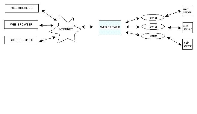
Since the Web emerged, it was enrolled to share 2D GIS data. At the current stage, there are two types of Web 2D GIS: server-side and client-side. The server side is based on connections to GIS servers by CGI scripts. In practice, the user requesting GIS information, activates a CGI script, which transforms the query to a GIS executable operation, processes the result in a form appropriate for display in a Web browser and delivers it to the client-site. The result is usually displayed as text or image in an HTML page. Examples of such access to GIS are VISA International (http://www.visa.com), MapQuest (http://www.mapquest.com). The major disadvantage is that interactivity on the client site is on a very low level: a new pan or zoom operation activates a new connection to the server. The apparent advantage is that all the computations are performed on the server side, which permits employment of existing GIS and DBMS servers.

The client-side GIS is realised following different approaches: plug-ins (helpers) and Java applets. The plug-ins are programs that enable the Web browser to read and visualise types of data not supported by HTML, i.e. they have to be installed permanently on the client site. Java applets are programs written in the Java language that reside on the server. They are delivered to the client site on user request and stay active for the time of their running. Since the processing of data is shifted to the client site, the possibility for the interaction and manipulation of data is greater. In general, Java applets are considered the more powerful approach that plug-ins, since the applet preserves most of the Web functionality, has a smaller size then an HTML page (the Java applet is a compiled program) and provides flexible means of visualising graphics (e.g. Java 3D). The often-mentioned disadvantage is the restriction of possible connection to one server, i.e. the server where the applet is launched. An example of a GIS plug-in is MapGuide (http://www.mapquide.com) and a Java based GIS is the ArcView Internet Map (http://www.ersi.com).

2.4.2 VRML: the Web standard for 3D visualisation

• enable development of computer programs to create, edit and maintain VRML (i.e. VR modellers)
• enable development of computer programs to visualise and navigate through VRML (i.e. VR browsers)
• encourage development of programs for the conversion of other graphics file formats into VRML (i.e. converters)
• provide means to use, combine and re-use dynamic 3D objects within VRML
• provide the ability to define new object types not explicitly defined in VRML
• enable implementation on a wide range of systems
• ensure interactive performance on a variety of computing platforms.

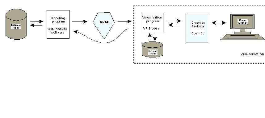
Designed for a standard Web protocol, VRML enables hyperlinks to other types of documents supported by the Web, e.g. movie, sound, HTML, VRML, and programs (CGI scripts, ECMAscripts and Java applets). It is capable of representing geometry, texture, materials, lighting, i.e. all the components of the scene (see Figure 2-4), as well as, the behaviour of objects and dynamics. The dynamics ranges from techniques to play complex animation to means of detecting user actions and consequent events. The ability to represent real worlds and their dynamics places VRML among the second-level modelling languages such as Open Inventor. Since the level of realism and dynamics that can be achieved in VRML is very high, the 3D models are called worlds or virtual worlds. Each world can be almost an unlimited composition of smaller worlds distributed on different servers all over the Web (see Chapter 4 for more details on VRML). All these features make VRML an attractive alternative for a front-end interface to 3D GIS data on the Web.

The 3D scene designed according to the VRML syntax is actually an ASCII file format, which can be read within any word processing software. In this text, the 3D scenes described in VRML will be referred to as worlds or documents (a general term for any data transferable on the Web). The term VRML model is frequently used to indicate individual objects (or groups of objects) that can be embedded in a world, e.g. a VRML model of a telephone. Visualisation software, i.e. a VR browser, displays the 3D model. We must distinguish between what can be described inside VRML files and what VR browsers are expected to supply. The VRML provides the parameters for scene description and the animation of objects while, the VR browser cares of rendering the scene and supplying the means to navigate through and interact with the model. Initially, the basic function of the VR browser, besides visualisation, was only real-time navigation, i.e. provision of virtual reality techniques: examine, fly-over, walk-through, pan, zoom. The second edition of VRML granted the VR browser new responsibilities related to various dynamics inside the scene. More details about the suite of VRML and VR browsers are given in Chapter 4.

The VR browser parses the VRML instructions in an internal model (scene graph) and ensures the rendering, the detection of user actions and the enabling of the hyperlinks. In the part of tasks related to the visualisation, the VR browser follows the traditional visualisation schema (compare Figure 2-3 and Figure 2-7). That is to say the modelling of VRML worlds does not require knowledge of rendering algorithms, windowing, device tracking or the design of tools for interaction. The separation between pure visualisation problems and the 3D modelling of worlds is considered by some authors a critical point that may save programming time and efforts, and ensure better concentration on specific tasks (see Nadeau 1997). The authors recommend VRML for systems, where the emphasis is more on the construction and analysis of the application models than on visualisation (see Sherman 1997).

2.5 Summary

The geometric characteristics of an object tend to define the object with respect to location in space, shape and size. These characteristics are closely related to abstractions about space and objects. The vector representation allows a more accurate description than the raster representation and therefore it is used for this research. The real objects are commonly associated with four types of objects, i.e. points, lines, surfaces and bodies. Spatial relationships are needed to perform a large variety of GIS functions. The spatial relationships can be represented by several methods; among them, topology is widely applied due to ensured neighbourhood information and invariance under topological transformations. The semantic characteristics of objects and the time are beyond the scope of this thesis and therefore are not discussed here.

Three stages of GIS data model design are distinguished, i.e. conceptual, logical and physical. The GIS can be developed from scratch and then the three design stages have to be completed. The GIS can also be built on an existing database management system, making use of already provided operations. The second approach will be adopted here. Therefore, only two stages are of particular interest for this thesis, i.e. conceptual and logical design. Conceptual design refers to the clarification of objects, their attributes and relations. In this respect, the object-oriented approach and its common principles facilitate the abstraction of real objects. The logical design then is related to mapping the selected components to the relational data model. This process can be favoured by the utilisation of conceptual models (ERM, IFO) that provide methods of describing objects and their relations, and of mapping onto the relational data model.

The user interface is a very important part of 3D GIS development. In general, 3D GIS implies an expensive task in each of its aspects, i.e. data collection, design and maintenance. Therefore the user interface has to permit comprehensive utilisation of the information. The advances in computer graphics offer new extended tools for the visualisation, interaction and manipulation of data, which have to be fully employed for 3D GIS. Queries and visualisation of spatial analysis have to be graphics-oriented rather then text-oriented whenever appropriate.

An important factor in a 3D GIS is remote access to the data. Recent developments on the Web, i.e. VRML make possible visualisation and interaction with 3D models. The exploration of the 3D worlds in the VR browsers ensures a certain level of virtual reality techniques. Existing VRML, HTML and other Web standards and software modules allow the development of GUI with limited effort, relying on some operations provided already by browsers. Therefore VRML and HTML will be employed as a front-end engine to the 3D GIS model.