The derivation of topological relations here is based on the framework provided by the 9-intersection model (see Egenhofer and Herring 1990). The comprehensive formal categorisation of spatial relations is completed upon the comparison of the nine intersections between topological primitives, i.e. interior, boundary and exterior of object. The relations that can be detected applying the framework are many more than the ones that exist in reality. Therefore, the identification of possible relations becomes an important issue. Several authors have completed studies on the possible topological relations; however, most of them refer to the 2D domain and only partially to the 3D domain. The spatial model proposed focuses on the 3D domain. Therefore the first part of this chapter elaborates on the derivation on feasible relations between simple objects and proposes a unified procedure for identification of relationships. A discussion on the completeness of the set of relations obtained, topologically equivalent configurations and the naming of the relations is presented.
The second part of the chapter illustrates the manner
of detecting any of the relations by the SSM. The number of operations
needed to detect any of relationships is discussed. The intention is to
evaluate of the "cost" of arc removal for spatial analysis. A final deliberation
draws conclusions on the suitability of SSM to identify spatial relations.
6.1.1 Negative conditions6.2 Topological relations supported by SSM
6.1.2 Possible relationsLine and line relations in IR6.1.3 Completeness of the obtained relations
Line and line relations in IR 2 and IR 3
Surface and line in IR 2
Surface and line in IR 3
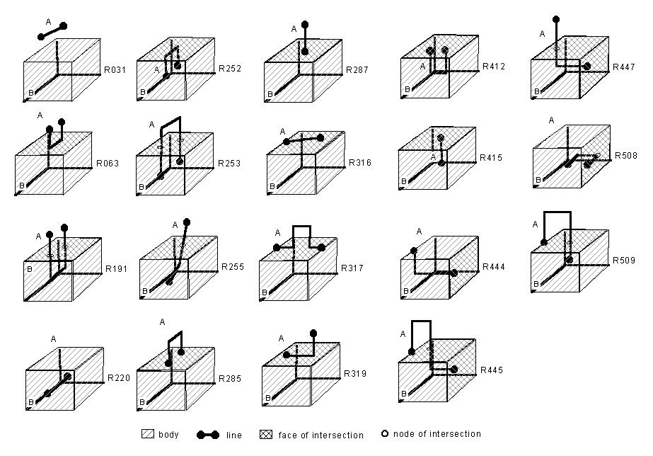
Body and line in IR 3
Surface and surface in IR 2
Surface and surface in IR 3
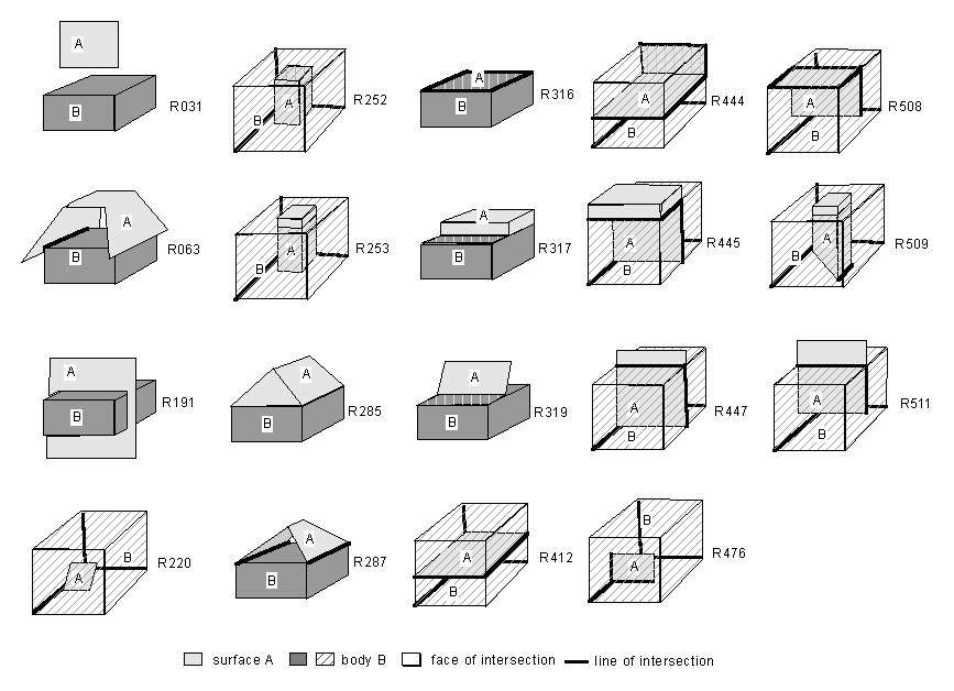
Body and surface in IR 3
Body and body in IR 3
Point and point
Point and any other object X
6.1.4 Topological equivalent spatial relationships
6.2.1 Point relations6.3 Usefulness of the decimal code
6.2.2 Line relationsLine and line6.2.3 Surface relations
Surface and line
Body and line
6.2.4 Body relationsBody and body
Body and surface
Suppose two simple spatial objects A and
B
(see Chapter 5) defined as non-empty sets
in the same topological space![]() ,
then their boundary, interior, exterior and closure will be denoted by
,
then their boundary, interior, exterior and closure will be denoted by ![]() and
and![]() (see
Chapter
2). The binary relation R(A,B)
between the two objects is then
identified by composing all the possible set intersections of the six topological
primitives, i.e.
(see
Chapter
2). The binary relation R(A,B)
between the two objects is then
identified by composing all the possible set intersections of the six topological
primitives, i.e.
![]() and
and ![]() ,
,
and detecting empty(![]() )
or non-empty (
)
or non-empty (![]() )intersections.
For example, if two objects have a common boundary, the intersection between
the boundaries is non-empty, i.e.
)intersections.
For example, if two objects have a common boundary, the intersection between
the boundaries is non-empty, i.e. ![]() ;
if they have intersecting interiors, then the intersection
;
if they have intersecting interiors, then the intersection![]() is
not empty, i.e.
is
not empty, i.e.![]() . The relation
R(A,B)
is a subset of the Cartesian product of
. The relation
R(A,B)
is a subset of the Cartesian product of ![]() ,
i.e.
,
i.e.![]() . The intersection between
the six primitives can be represented as an ordered set given by a 3
. The intersection between
the six primitives can be represented as an ordered set given by a 3 ![]() 3
intersection matrix, i.e.
3
intersection matrix, i.e.
Since each set intersection can have either the empty or non-empty value, different "patterns" of the 9-intersection matrix define different relations. For example, the relation defined above is disjoint.
For simplicity, instead of the matrix representation,
a line representation of all the intersections will be used in the following
text. Furthermore, the set intersections equal to the empty set will be
denoted by 0 and the non-empty intersections by 1. Thus, each relation
(being a sequence of 0 and 1) corresponds to a binary number, which can
be transformed to a decimal number (see Kufoniyi 1995). For example, the
relation between objects with non-intersecting closures (referring to the
matrix representation above) can be represented as 000011111, which is
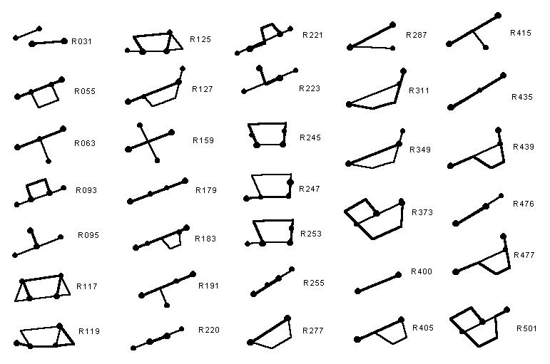
the decimal number 31. It will be denoted as a decimal code R031.
It is apparent that different ordering of the intersections between topological
primitives will result in a different decimal code. In this text, we will
use the order shown in Table
6-1. The benefit of this manner is that the nine intersections can
be separated into two general groups, which will be denoted as closure
intersections and exterior intersections.
The closure intersections
represent the 4-intersection model built on the mutual intersections of
two topological primitives (interior and boundary), i.e.![]() ,
, ![]() ,
,![]() and
and ![]() . The closure intersections
are positioned to the left side of the intersection between objects' exteriors,
i.e.
. The closure intersections
are positioned to the left side of the intersection between objects' exteriors,
i.e. ![]() The exterior intersections
are the four intersections between the exteriors and closure, i.e.
The exterior intersections
are the four intersections between the exteriors and closure, i.e.![]() ,
, ![]() ,
, ![]() and
and ![]() .
They are placed on the right of the intersection between both exteriors.
Since the set intersection
.
They are placed on the right of the intersection between both exteriors.
Since the set intersection![]() is
constantly non-empty for the defined spatial model (see Chapter
5), it "acts" as a delimiter between closure and exterior intersection.
The advantage of the linear ordering and corresponding decimal coding is
threefold:
is
constantly non-empty for the defined spatial model (see Chapter
5), it "acts" as a delimiter between closure and exterior intersection.
The advantage of the linear ordering and corresponding decimal coding is
threefold:
| R031 | 0 | 0 | 0 | 0 | 1 | 1 | 1 | 1 | 1 |
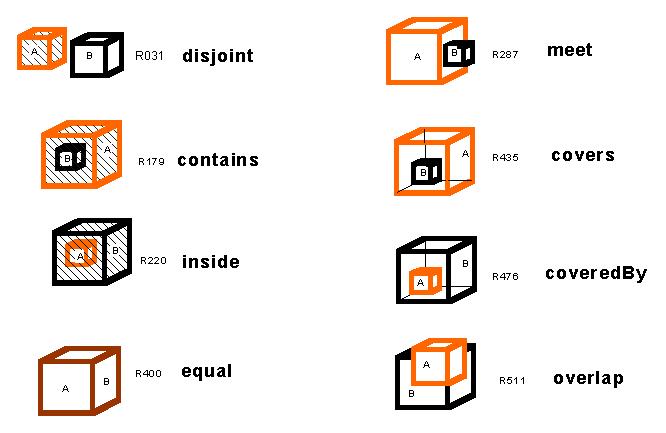
The theoretical number of all the relations that can be derived from the matrix is 29, i.e. 512 relations. However, only a small number of them can be realised in reality. For example, the only possible configurations between two bodies in 3D or two simple surfaces in 2D are only eight (see Figure 6-6 and Figure 6-5). The identification of possible relations is as important as the identification of the relations. From the implementation point of view, the elimination of impossible relations will reduce the number of combinations to be examined and thus improve the performance of the spatial model.
The way to specify possible relations is based on the
elimination of impossible ones. To eliminate impossible relations, negative
conditions are composed. Some intersections (or a combination of intersections)
between topological primitives can never occur in reality, and all the
relations that contain these intersections (or the combination) can be
securely excluded. For example, the definitions of SSM ensure that the
intersection ![]() is non-empty
for any two objects. This can be expressed verbally as a negative condition
"the intersection
is non-empty
for any two objects. This can be expressed verbally as a negative condition
"the intersection ![]() is always
non-empty" and represented according to our notations as:
is always
non-empty" and represented according to our notations as:
| CX | | | | | 0 | | | | |
On the basis of the 9-intersectin model and following the "elimination-of-impossible-relations" approach, several authors have identified relations between points, lines, surfaces and bodies. Egenhofer and Herring 1992, Egenhofer and Franzosa 1991, Molenaar et al 1994, Kufoniyi 1995 investigate relationships between spatial objects in IR 2. Egenhofer 1995 presents relations among body objects in IR 3. De Hoop et al 1993 report a method to distinguish between multidimensional objects in IR 3. The outlined possible relations between objects are usually illustrated with drawings, i.e. sketches of possible object configurations. Bric 1993 investigates the largest combinations of objects, following the condition approach for elimination introduced by van der Meij 1992. The study, however, does not provide drawings of the elected configurations. The different conditions used for objects in 2D and 3D space, as well as the lack of a complete list with drawings for all the possible configurations, have motivated the study presented here.
The analysis of the negative conditions used by the authors has revealed a significant variation in the number of conditions. Egenhofer and Herring 1992 present 23 negative conditions for relations in 2D space, i.e. relations between points, lines and surfaces. To cover the 3D situations, 15 more conditions have been added by van der Meij 1992. Bric 1993 operates with 40 conditions as 30 of them are used to derive the relations between simple GO in 3D space and 10 to derive the relations between CnsO. In general, the results, i.e. the elected possible relations, can be equivalent despite the different negative conditions applied. However, the selection of a minimal set of negative conditions is quite challenging.
The verbal description of the negative conditions varies as well. Since most of the conditions are built on the "if then" construction, the conditional (if) and the consequent (then) part of the statement could be reversed. The variety of expressions increases with the number of intersections involved. For example, the condition C15 (see below) can be represented in at least two more ways depending on which intersection will be mentioned in the "if" part. It may be written as:
The study on the possible relations has two phases. First, the set of negative conditions is presented. It consists of a computation of relations and verification by drawings. Second, the obtained relations are investigated for completeness. A second approach based on analysis of possible exterior intersections, is elaborated.
The spatial objects considered are simple objects without holes, tunnels and self-intersecting parts. The conditions are derived from the topological primitives as they are defined in the spatial model (Chapter 5). No special conditions related to some specific characteristics of the spatial model are included. Since the spatial objects considered in the model are the GO named point, line, surface and body, the corresponding notations P, L, S and B will be used to represent the relations. For example, R(L,S) means that the binary relation concerns line and surface as the line is the first object. The relation R(S,L) is the converse relation, which is referred to by the vice versa part of the condition .
In general, the negative conditions are composed on the basis of possible or non-possible intersections of topological primitives (i.e. interior, boundary and exterior) of two objects. In reality, the intersections between the topological primitives depend on three parameters: the dimension of the objects, the dimension of the space (which is used to define a co-dimension of the object) and the type of boundary (connected or disconnected). For example, the boundary of a surface in IR 2 cannot intersect with the interior of another surface without crossing the boundary. However, this is not the case in IR 3. Due to higher space dimension, the boundary of the surface can intersects with the interior of the other surface. The three parameters, however, cannot be used to define straightforward negative conditions. Unfortunately, each configuration of objects has different parameters (see Table 6-2). For example, the relationships between lines in IR2 are realised under the following parameters: the two objects have an object dimension one, the space dimension is two and both objects have disconnected boundaries. The parameters for the relationships between surface and surface in IR3 are different: the object's dimension is two, the space dimension is three and the boundaries of the surfaces are connected. However, many of the negative conditions are derived on the basis of one or another parameter that still permits a certain grouping.
Table 6-2: Parameters influencing the possibility of relations
| Parameters | Dimension of objects | Co-dimension of objects | Connectivity of boundaries | |||
| Objects | First | Second | First | Second | First | Second |
| R(P,P) in 1D, 2D, 3D | 0 | 0 | 1,2,3 | 1,2,3 | C | C |
| R(P,X) in 1D, 2D, 3D | 0 | 1,2,3 | 1,2,3 | 0,1,2 | C | D,C |
| R(L,L) in 1D | 1 | 1 | 0 | 0 | D | D |
| R(L,L) in 2D | 1 | 1 | 1 | 1 | D | D |
| R(L,L) in 3D | 1 | 1 | 2 | 2 | D | D |
| R(L,S) in 2D | 1 | 2 | 1 | 0 | D | C |
| R(L,S) in 3D | 1 | 2 | 2 | 1 | D | C |
| R(L,B) in 3D | 1 | 3 | 2 | 0 | D | C |
| R(S,S) in 2D | 2 | 2 | 0 | 0 | C | C |
| R(S,S) in 3D | 2 | 2 | 1 | 1 | C | C |
| R(S,B) in 3D | 2 | 3 | 1 | 0 | C | C |
| R(B,B) in 3D | 3 | 3 | 0 | 0 | C | C |
1. Conditions for binary relations between any objects: R(L,L) in IR , R(L,L), R(S,S), R(L,S) and R(S,L) in IR 2, R(L,L), R(S,S), R(B,B), R(L,S), R(L,B), R(S,B), R(S,L), R(B,L), R(B,S) in IR 3.
C1. The exteriors of two objects always intersect, i.e.
| R(A,B) | |||||||||
| C1 | | | | | 0 | | | | |
C2. If As boundary intersects with Bs exterior then As interior intersects with Bs exterior too and vice versa, i.e.
| R(A,B) | |||||||||
| C2a | | | | | | | | 1 | 0 |
| C2b | | | | | | 1 | 0 | | |
C3. As boundary intersects with at least one part of B and vice versa, i.e.
| R(A,B) | |||||||||
| C3a | 0 | | 0 | | | | | 0 | |
| C3b | 0 | | - | 0 | | 0 | | | |
After the first three negative conditions, the number of possible binary relations is reduced to 104 for spatial objects with equal dimensions and to 160 between spatial objects with different dimensions.
2. Conditions for binary relations between spatial objects of equal dimension: R(L,L) in IR , R(S,S) and R(L,L) in IR 2, R(L,L), R(S,S) and R(B,B) in IR 3.
C4. If both interiors are disjoint then As interior intersects with Bs exterior and vice versa, i.e.
| R(A,B) | |||||||||
| C4a | | 0 | | | | | | | 0 |
| C4b | | 0 | | | | | 0 | | |
C5. If As interior intersects with Bs boundary, then it must also intersect with Bs exterior and vice versa, i.e.
| R(A,B) | |||||||||
| C5a | | | | 1 | | | | | 0 |
| C5b | | | 1 | | | | 0 | | |
One part of the condition is true for the relations between objects with different dimension as well, i.e. C5a for relations when the first object A has the higher dimension. However, it is not necessary to use this due to the more restrictive condition C6.
3. Conditions for binary relations between objects of different dimensions: R(S,L), R(L,S), R(B,L), R(L,B), R(B,S), and R(S,B).
C6. The closure of A (the object with the higher dimension) always intersects with the exterior of B, i.e.
| R(A,B) | |||||||||
| C6a | | | | | | | | | 0 |
| C6b | | | | | | | | 0 | |
| C6c | | | | | | 0 | | | |
| C6d | | | | | | | 0 | | |
4. Conditions for binary relations between objects of different dimensions and at least one of the objects has a zero co-dimension:R(L,S) and R(S,L) in IR 2 ,R(L,B) R(S,B), R(B,L) and R(B,S) in IR 3.
C7. The interior of A always intersects with at least one of the three topological primitives of B and vice versa, i.e.
| R(A,B) | |||||||||
| C7a | | 0 | | 0 | | | | | 0 |
| C7b | | 0 | 0 | | | | 0 | | |
5. Conditions for binary relations between objects when at least one of the objects has a zero co-dimension: R(L,L) in IR , R(S,S), R(L,S) and R(S,L) in IR 2, R(L,B) R(S,B), R(B,L), R(B,S), R(B,B) in IR 3.
C8. If both interiors are disjoint, then As boundary cannot intersect with Bs interior, i.e.
| R(A,B) | |||||||||
| C8a | | 0 | 1 | | | | | | |
| C8b | | 0 | | 1 | | | | | |
C9. If As interior intersects with Bs interior and exterior, then it must intersect with Bs boundary too and vice versa, i.e.
| R(A,B) | |||||||||
| C9a | | 1 | | 0 | | | | | 1 |
| C9b | | 1 | 0 | | | | 1 | | |
6. Conditions for binary relations where at least on of the objects has disconnected boundaries: R(L,L), R(S,L), R(S,L), R(B,L), R(L,S), R(L,S), R(L,B).
The next condition raises when at least one of the objects has disconnected boundaries (i.e. it is valid for lines). The dimension of the second object and the co-dimension does not influence the condition. Since the line boundary consists of two disconnected nodes, it can intersect at most with two topological primitives, i.e.
C10. As boundary always intersects withat most two parts of B and vice versa, i.e.
| R(A,B) | |||||||||
| C10a | 1 | | | 1 | | 1 | | | |
| C10b | 1 | | 1 | | | | | 1 | |
7. Conditions for binary relations between objects with connected boundaries and at least one of the objects has a zero co-dimension: R(S,S) in IR 2, R(S,B) and R(B,S), R(B,B) in IR 3.
C11. If As boundary intersects with Bs interior and exterior, then it must intersect with Bs boundary too, i.e.
| R(A,B) | |||||||||
| C11a | 0 | | 1 | | | | | 1 | |
| C11b | 0 | | | 1 | | 1 | | | |
8. Conditions for binary relations between objects with equal dimensions and zero co-dimensions: R(L,L) in IR , R(S,S) in IR 2 and R(B,B) in IR3.
The continuity of the spatial objects and the space they are embedded in, restricts the interior and boundary to mutually either intersect, or coincide or be disjoint. In the case of intersection and disjoint, a subset of at least one boundary (interior) always intersects with the opposite exterior (continuity of spatial objects).
C12. If both boundaries do not coincide, then at least one boundary must intersect with the opposite exterior, i.e.
| R(A,B) | |||||||||
| C12 | 0 | | | | | 0 | | 0 | |
| R(A,B) | |||||||||
| C13 | | 0 | | | | 0 | | 0 | |
| R(A,B) | |||||||||
| C14a | | | | | | | | 0 | 1 |
| C14b | | | | | | 0 | 1 | | |
C15. If As interior is a subset of Bs interior, then As exterior intersects with both Bs boundary and Bs interior and vice versa, i.e.
| R(A,B) | |||||||||
| C15a | | | | | | 0 | 1 | | 0 |
| C15b | | | | | | | 0 | 0 | 1 |
C16. If As interior intersects with Bs boundary but As boundary do not intersect with Bs interior, then As boundary must intersect with Bs exterior and vice versa, i.e.
| R(A,B) | |||||||||
| C16a | | | 0 | 1 | | | | 0 | |
| C16b | | | 1 | 0 | | 0 | | | |
10. Conditions for binary relations objects of the same dimension with connected boundaries and non-zero co-dimension: R(S,S) in IR3.
As was mentioned, self-intersecting spatial objects are not allowed in the spatial model and therefore they are excluded from the list of possible relations The conditions listed below eliminate closed surfaces (see Figure 6-1).
C17. If As interior does not intersect with Bs boundary and As boundary does not intersect with Bs interior, then both boundaries either intersect or not with both exteriors, i.e.
| R(A,B) | |||||||||
| C17a | | | 0 | 0 | | 1 | | 0 | |
| C17b | | | 0 | 0 | | 0 | | 1 | |
| R(A,B) | |||||||||
| C18a | | 1 | 1 | 1 | | 0 | | 0 | |
| C18b | 1 | | 1 | 1 | | 0 | | 0 | |
| R(A,B) | |||||||||
| C19a | 1 | 1 | 1 | 1 | | | | 0 | |
| C19b | 1 | 1 | 1 | 1 | | 0 | | | |
C20. If As interior intersects with Bs boundary but not Bs interior, then Bs interior must intersect with As exterior, i.e.
| R(A,B) | |||||||||
| C20a | | 0 | | 1 | | | 0 | | |
| C20b | | 0 | 1 | | | | | | 0 |
C21. If the boundary of B intersects with the boundary of A but the interior of B does not intersect with both the interior and boundary of B, then the interior must intersect with the exterior of A, i.e.
| R(A,B) | |||||||||
| C21 | 1 | 0 | 0 | | | | 0 | | |
| C21b | 1 | 0 | | 0 | | | | | 0 |
12. Conditions for binary relations between objects of equal dimension, non-zero co-dimension and disconnected boundaries: R(L,L) in IR 2 and IR 3.
C22. If A's boundary is a subset of B's boundary, then the two boundaries coincide and vice versa, i.e.
| R(A,B) | |||||||||
| C22a | 1 | | 0 | | | 1 | | 0 | |
| C22b | 1 | | | 0 | | 0 | | 1 | |
Let ![]() ,
, ![]() and
and ![]() .
This implies that
.
This implies that ![]() . Since
the cardinality of the two sets is equal, then either
. Since
the cardinality of the two sets is equal, then either ![]() and
and ![]() or
or ![]() and
and ![]() .
.
13. Conditions for binary relations between objects with at least one empty interior: R(P,P), R(P,L), R(P,S), R(P.B), R(L,P), R(S,P), R(B,P).
C23. If A's interior is the empty set, all the intersections between A's interior and B's topological primitives will be the empty set and vice versa, i.e.
| R(A,B) | |||||||||
| C23a | | 1 | | | | | | | |
| C23b | | | | 1 | | | | | |
| C23c | | | | | | | | | 1 |
| C23d | | | 1 | | | | | | |
| C23e | | | | | | | 1 | | |
| R(A,B) | |||||||||
| C24a | 1 | | 1 | | | | | | |
| C24b | 1 | | | | | | | 1 | |
| C24c | | | 1 | | | | | 1 | |
| C24d | 1 | | | 1 | | | | | |
| C24e | 1 | | | | | 1 | | | |
| C24f | | | | 1 | | 1 | | | |
| R(A,B) | |||||||||
| C25a | 0 | | | | | 0 | | | |
| C25b | 0 | | | | | | | 0 | |
The negative conditions defined above are applied to identify topological binary relations between simple spatial objects regardless of the space in which they are embedded (i.e. IR, IR 2, or IR 3 ).. A program written in J (see http://www.jsoftware.com)computes the possible relations.
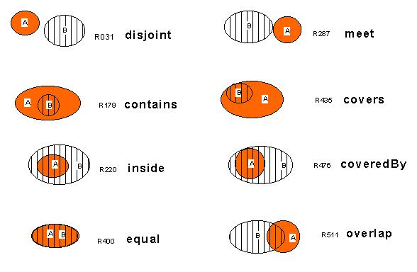
Figure 6-2: Line and line in IR : 8 relations
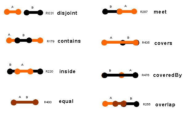
Line and line relations in IR: Lines are spatial objects with disconnected boundaries and connected interior. Embedded in IR , their co-dimension is zero (see Table 6-2). Therefore the following conditions have to be applied: C1, C2a, C2b, C3a, C3b, C4a, C4b, C5a, C5b C8a, C8b, C9a, C9b, C10a, C10b, C12, C13, C14a and C14b. Since the two objects have the same dimension both parts of all the conditions have to be used. The number of identified possible relations is eight (see Figure 6-2 and Appendix 3) and they are given the names: disjoint, contains, inside, equal, meet, covers, coveredBy, overlap.
Line and line relations in IR 2 and IR 3: The negative conditions for R(L,L) in IR 2 and IR 3 are C1, C2a, C2b, C3a, C3b, C4a, C4b, C5a, C5b, C10a, C10b, C15a, C15b C16a, C16b, C22a and C22b. Lines embedded in IR 2 or IR 3 have disconnected boundaries and connected interior but the co-dimension is non-zero. Therefore, the negative conditions that have to be applied belong to the following groups: conditions for all objects, conditions for objects of the same dimension, conditions for objects with disconnected boundaries, conditions for objects of the same dimension and non-zero co-dimension, and conditions for line and line relations in IR 2 and IR 3. The number of all the relations is 33. Figure 6-3 presents a geometric interpretation of all the relations. Egenhofer and Herring 1992 report the same number of relations; however the number of conditions with all their parts is 20. Molenaar et al 1994 report 22 relations. Drawings with their possible geometric configurations are shown in Kofuniyi 1995.
Surface and line in IR 3: Surface and line embedded in IR 3 have the same properties as surface and line in IR 2, however the co-dimension is non-zero (see Table 6-2). The non-zero co-dimension permits 12 more configurations than in IR 3, i.e. the total number of all the possible relations is 31 (see Figure 6-4). The conditions used for the relation R(S,L) are: C1, C2b, C3b, C6a, C6b, C10a C20a and C21a. Bric 1993 obtains the same binary relations but applying 14 conditions (counting all the parts of the condition.
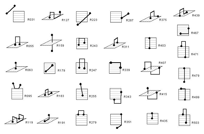 |
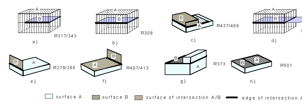
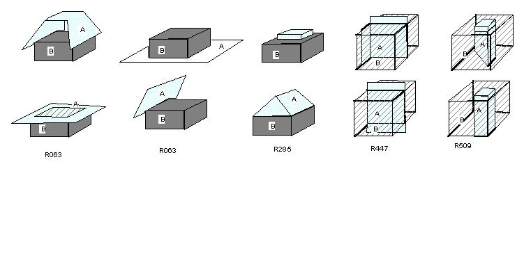
Figure 6-7: Surface and surface in IR 3 : 38 relations
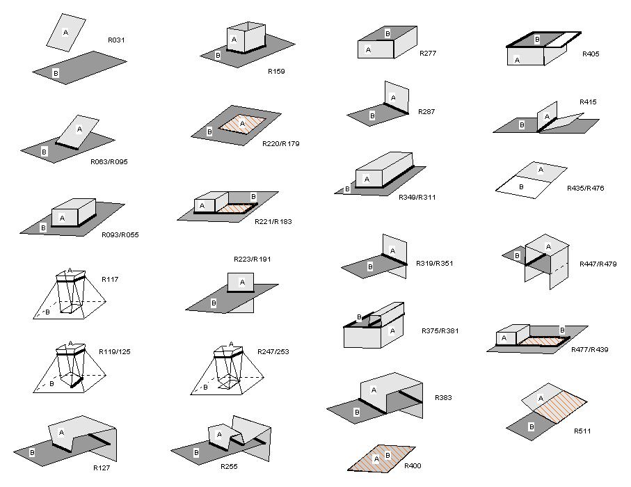
Surface and surface in IR 3: The possible relations between surface and surface are determined by the following properties: equal dimension, connected boundaries and non-zero co-dimension. Since the co-dimension is greater than zero, the surfaces have the "freedom" to touch their interiors without intersection of boundaries and therefore more relations are obtained. Thus, only the first five conditions, i.e. C1, C2a, C2b, C3a, C3b, C4a, C4b, C5a and C5b are considered of all the ones used for R(S,S) in IR 2. In addition, C15a, C15b, 16a, 16b, the four parts of C17, C18a, C18b, C19a and C19b, must be applied to avoid self-intersecting boundaries (see Figure 6-1). The number of obtained relations is 38 (see Figure 6-7 and Appendix 3).
Bric 1993 is the only author reporting the matrices with relations between surfaces in IR 3 (De Hoop et al 1993 give only the number of relations 47). The obtained relations however are different. Relations R117, R159, R277 and R405 are not elected as possible and 12 new relations are reported, which (in our judgement) require self-intersecting surfaces. The 12 new relations are R279, R285, R317, R343, R407, R412, R433, R445, R471, R501, R503 and R509. Relations R279 and R285 could not be interpreted with any geometric configuration between simple surfaces; relations R317, R343, R407, R413, R433, R445 and R471 can be realised by self-intersection of one of the surfaces (see Figure 6-1).
 |
 |
Point and point: Since the points are objects with empty interior and equal dimensions, the conditions that to be applied are C1, C23a, C23b, C23c, C23d, C23e, C24b, C24e, C25a and C25b. These conditions eliminate 510 relations and leave only two, i.e. equal and disjoint.
Point and any other object X: R(P,X), R(X,P). The relations between a point and any other object are only three, i.e. a point can be disjoint, lay on the boundary of an object or on its interior. These configurations can be obtained by applying conditions for R(P,X): C1, C3a, C6c, C6d C23a, C23b, C23c, C24a, C24b, C24c and C25a.The reverse relations R(X,P) require the conditions: C1, C3b, C6a, C6b C23a, C23d, C23e, C24d, C24e, C24f and C25b.
All the possible relations computed on the basis of the negative conditions are given in Appendix 3. The total number of all the binary relations between simple objects according to the 9-intersection model is 69. Table 1 (Appendix 3) contains the binary relations and the corresponding decimal codes. The relations are sorted in an ascending order according to the decimal code. The decimal coding places relations with less non-empty intersections between interior and boundary at the top of the table and relations with more non-empty intersections at the bottom of the table. Since the first four columns represent the closure intersections, the 16 relations according to the 4-intersection model can clearly be distinguished from the additionally identified ones according to the 9-intersection model. The relations in the table are subdivided into 16 groups corresponding to the 16 closure intersections. Four closure relations have converse relations, i.e. the relations of groups 2&3, 6&7, 10&11 and 14&15. Such relations can be represented by one geometric configuration of spatial objects (e.g. Figure 6-6 and Figure 6-7).
6.1.3 Completeness of the obtained relations
The completeness of the relations is of great importance to the development of algorithms and operations to identify relations. As can be observed from the sketches, many relations of spatial objects belong to only one group of relations (see also Appendix 3). For example, surface and line can relate according to the relation R375 (see Figure 6-4). The relation belongs to group 12. Since the configuration does not have another relation from this group, the closure intersection is sufficient to conclude in support or against the relation. Thus the operations related to inspection of exterior intersection can be omitted. The benefit will be the improved performance of the spatial queries based on this topological relation. Such shortening of the query process is affordable only if the completeness of the possible relations is ensured.
The procedure followed above relies on the correct composition of negative conditions. Drawings of the possible configurations of spatial objects are used for final approval of the resulting relations. The approach has the weak characteristic that it cannot control the strictness of the negative conditions. Some risk exists that a condition might be too strict and cause elimination of configurations that are realisable in reality. The relaxed conditions that leave relations can be identified as wrong by the final proof (sketches of spatial objects) afterwards. The final proof, however, cannot detect omission of possible relations. For example, the conditions presented by Bric 1993 for the surface and surface configuration eliminate four possible intersections between simple, non-closed surfaces.
This section investigates the relations from a different viewpoint, i.e. the emphasis is on the possible combinations between the 16 closure intersections and the 16 exterior intersections. The dimension of objects and the dimension of the embedding space are not of primary consideration.
Since the exterior of spatial objects is defined as the set difference between the universe and the closure, the intuitive expectation is that there are a very limited number of possible intersections. The exterior of the object A cannot be restricted to intersect only with the boundary or interior of the object B. The exterior of A is an open set (by definition) while the closure of B is a closed set (by definition), which implies that they never can coincide. This means that always there is either A's exterior intersecting with other parts of B or B's exterior intersecting with a part of A. Thus we can specify a number of impossible exterior intersections for any object regardless of dimensions and co-dimensions. The impossible intersections are differentiated by the following four statements:
1. The exterior of A never intersects with only B's boundary or interior and vice versa, which eliminates the following exterior combinations.
| E9 | | | | | | 1 | 0 | 0 | 0 |
| E5 | | | | | | 0 | 1 | 0 | 0 |
| E3 | | | | | | 0 | 0 | 1 | 0 |
| E2 | | | | | | 0 | 0 | 0 | 1 |
| E7 | | | | | | 0 | 1 | 1 | 0 |
| E10 | | | | | | 1 | 0 | 0 | 1 |
The elimination of all the six impossible combinations
reduces the possible exterior interceptions to 10. Thus, the number of
candidate relations according to the 9-intersection model (considering
the intersection ![]() ) is decreased
to 112.
) is decreased
to 112.
The next two statements are again true for any configurations of objects, however they have some exceptions:
3. If A's exterior intersects with B's boundary, it must also intersect with B's interior and vice-versa (except point objects), i.e. the following exterior intersections do not exist.
| E11 | | | | | | 1 | 0 | 1 | 0 |
| E12 | | | | | | 1 | 0 | 1 | 1 |
| E15 | | | | | | 1 | 1 | 1 | 0 |
Exceptionally, the above exterior intersections are possible only for point objects. Since a point object does not have any interior (by definition), the intersections cannot be composed and they are assumed empty. Hence, these exterior intersections must appear only once in the entire list of possible relations.
4. At least one exterior intersects with the closure of the opposite object (except for coinciding objects), i.e. the following exterior intersection is impossible.
| E1 | | | | | | 0 | 0 | 0 | 0 |
The 10 combinations of exterior intersections considered so far leave 101 candidate relations out of the initial 255. The exterior intersections, which are still not analysed, are six in total. Four of them are mutually converse, i.e. E4&E13 and E8&E14, and therefore they are regarded together.
The first combination (E4&E13) means that one of the objects is inside the other object, i.e. the boundary and the interior do not intersect with the exterior of the opposite object. It is possible only if there is at least one intersection between the boundary of one of the objects and the interior of the other object. Analysis of this pattern shows three possibilities:
| E4 | | | | | | 0 | 0 | 1 | 1 |
| E13 | | | | | | 1 | 1 | 0 | 0 |
2. A close intersection can be combined only with one
of the two exterior intersections. Such closure intersections must have
one non-empty ![]() or
or ![]() intersection and at least one empty
intersection and at least one empty![]() or
or ![]() intersection. The closure
relations that represent these intersections are 2&3, 6&7, 10&11.
intersection. The closure
relations that represent these intersections are 2&3, 6&7, 10&11.
3. Closure relations can be combined with both exterior
intersections. The case is possible when either both the set intersections![]() and
and ![]() or the three intersections
or the three intersections ![]() ,
,![]() and
and ![]() are non-empty. The
closure relations that fulfil the first statement are 13, 14, 15 and 16
and closure intersections 8 and 9 satisfy the last two statements. Thus
the number of possible relations is 18 (4x0+6x1+4x2+2x2=18).
are non-empty. The
closure relations that fulfil the first statement are 13, 14, 15 and 16
and closure intersections 8 and 9 satisfy the last two statements. Thus
the number of possible relations is 18 (4x0+6x1+4x2+2x2=18).
| E8 | | | | | | 0 | 1 | 1 | 1 |
| E14 | | | | | | 1 | 1 | 0 | 1 |
| E6 | | | | | | 0 | 1 | 0 | 1 |
The last pattern, i.e. all the set intersections are non-empty, can be combined with all the 16 possibilities of closure intersection, which gives 16 relations.
| E16 | | | | | | 1 | 1 | 1 | 1 |
| Number | |||||
| E1 | 0 | 0 | 0 | 0 | 2 |
| E2 | 0 | 0 | 0 | 1 | 0 |
| E3 | 0 | 0 | 1 | 0 | 0 |
| E4 | 0 | 0 | 1 | 1 | 9 |
| E5 | 0 | 1 | 0 | 0 | 0 |
| E6 | 0 | 1 | 0 | 1 | 6 |
| E7 | 0 | 1 | 1 | 0 | 0 |
| E8 | 0 | 1 | 1 | 1 | 12 |
| E9 | 1 | 0 | 0 | 0 | 0 |
| E10 | 1 | 0 | 0 | 1 | 0 |
| E11 | 1 | 0 | 1 | 0 | 1 |
| E12 | 1 | 0 | 1 | 1 | 1 |
| E13 | 1 | 1 | 0 | 0 | 9 |
| E14 | 1 | 1 | 0 | 1 | 12 |
| E15 | 1 | 1 | 1 | 0 | 1 |
| E16 | 1 | 1 | 1 | 1 | 16 |
| Total | 69 |
If A's exterior intersects with B's interior but not with the boundary, then B's exterior must intersect at least with A's interior and vice versa.
| ECa | | | | | | 0 | 1 | | 0 |
| ECb | | | | | | | 0 | 0 | 1 |
The literal expression cannot be found in the list
of conditions given with the first approach; however, the combination of
restrictive empty non-empty intersections is equivalent to the ones given
in the condition C15. C15 in the first approach has a limited range, i.e.
it is applied to the relations between only two configurations of objects
R(L,L) in IR 2 and R(S,S) in IR 3.
According to the analysis of exterior intersection, the condition EC must
be applied to all the binary relations between any types of object, regardless
of dimensions and connectivity of boundaries. This example is yet another
illustration of the different possibilities to compose negative conditions.
6.1.4 Topological equivalent spatial relationships
Although the 9-intersection model recognises more relations then the 4-intersection model, it is still not sufficient to describe all the possible ones existing in reality. The basic concept of the model is the detection of empty or non-empty set intersection between the topological primitives. In practice, the set intersection can be an empty or non-empty set. However, if the intersection is a non-empty set, further investigation of the set intersection is not provided. For example, referring to SSM, the non-empty set intersections might be a node, a set of nodes, a face or a set of faces. Moreover, the set may have disconnected boundaries or disconnected interiors or both. Another factor that influences the geometric representations is the number and position of the disconnected sets. The variety of non-empty intersections implies that the object configurations performing the same topological relation vary as well. Configurations of objects that reveal the same topological relation are known as topologicallyequivalent. Figure 6-10 and Figure 6-11 show topologically equivalent surface and surface compositions and Figure 6-12 portrays some equivalent body and body interactions.
Egenhofer and Franzosa 1994 present a comprehensive approach to distinguish topologically equivalent relations between regions in 2D space, estimating the dimension of the set intersections, connectivity, number and order of disconnected sets and the sequence of boundary and boundary components. The framework is built on the 4-intersection model.
Here, we propose an idea to refine topologically equivalent relations in 3D, judging the non-empty intersections obtained. The estimation of the intersections is completed on: 1) the intersection set between the two objects and 2) the non-empty intersections according to the 9-intersection model. To illustrate the idea, we will focus on the relation R223 between surface and surface (see Figure 6-10). The relation R223 is represented by seven non-empty and two empty set intersections (see Table 6- 4). To evaluate all the non-empty intersections, three parameters are considered: the dimension of the obtained intersections, connectivity and the number of disconnected intersections. The following notations are used: c-connected set, d-disconnected set, cb-connected boundary set; db-disconnected boundary set, ci-connected interior set, di-disconnected interior set. The type of intersections is denoted by n-a node, nn-a set of nodes, f-a face, ff-a set of faces.
Table 6-4: Properties of the set intersections for relation R223
| Intersection
set |
||||||||||
| R223 | 0 | 1 | 1 | 0 | 1 | 1 | 1 | 1 | 1 | |
| A | nn,db,ci | - | nn, c | nn, d | - | - | nn, c | ff, d, 1 | nn, d, 1 | ff, d, 1 |
| B | f,cb,ci | - | f, c | nn, c | - | - | nn, c | ff, d, 1 | nn, c | ff, c |
| C | nn,db,ci | - | nn, c | n, d, 1 | - | - | nn, c | ff, d, 1 | nn, d, 1 | ff, d, 1 |
| D | nn,db,ci | - | nn, c | n, d, 1 | - | - | nn, c | ff, d, 1 | nn, d, 1 | ff, d, 1 |
| E | nn,db,di | - | nn, d, 1 | nn, n, d, 2 | - | - | nn, c | ff, d, 2 | nn, c | ff, d, 1 |
| F | nn,db,di | - | nn, d, 1 | n, d, 3 | - | - | nn, c | ff, d, 2 | nn, d, 1 | ff, d, 2 |
| G | nn,cb,ci | - | nn, c | nn, c | - | - | nn, c | ff, d, 2 | nn, c | ff, d, 1 |
| H | f,cb,ci | - | f, c | nn, c | - | - | nn, c | Ff, d, 1 | nn, c | ff, c |
The column "intersection set" contains the characteristics of the set obtained as intersection of objects. The remaining columns contain characteristics of the set intersection between topological primitives of the objects. Since the "intersection set" is regarded as a new object (surface, line, point), a distinction between connectivity of boundary and interior is provided.
The first step distinguishes between three groups of cases: 1) b and h, 2) a, c, d, g, and 3) e, f (see Table 6-4). The second step allows further refinement between some of the cases. As can be observed from the table, some geometric configurations remain topologically equivalent, e.g. b and h, c and d. However, they cannot be identified as different relations only on the basis of the three topological primitives and set theory operations.
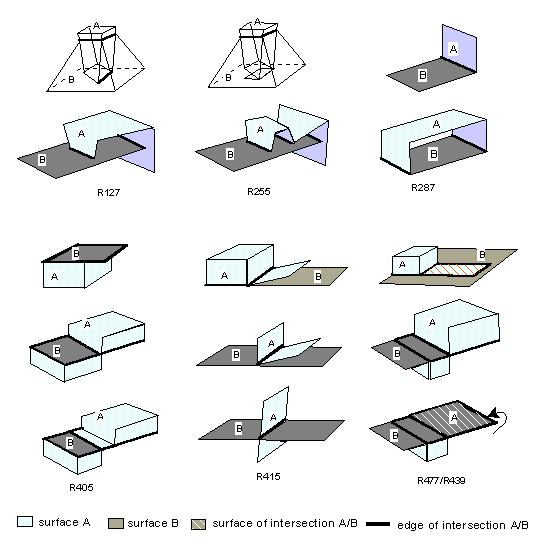
Figure
6-11: Surface relations topologically equivalent to R127, R255, R287, R405,
R415 and R477/R439
Figure
6-12 : Topological equivalent relations between body and body
The spatial model proposed in this thesis lacks a 1D constructive primitive, i.e. arc, which may have impact on the detection of the relations at implementation level. This section demonstrates availability of all the relations in the spatial model.
The binary relations are identified on the basis of empty or non-empty intersections of the three topological primitives. The definitions of spatial objects, however, are based on boundary description, i.e. the boundary is materialised by sets of nodes. This implies that the exterior and, in some cases, the interior are not explicitly detectable. Although many configurations of objects do not require considerations of exterior, some are distinct on the basis of the mutual position of closures and exteriors. In general, if the relations that are valid for a particular object configuration belong to one group, e.g. surface and surface line and line in IR 3 (see Appendix 3), then exterior intersections are needed. Therefore, it is essential to clarify the tracking the exterior and thus identifying the intersections. As was shown, the number of combinations of empty non-empty exterior intersections possible in reality is 10, as three of them can occur only for point objects and one exists for equal objects. The relations that appear between point objects are exceptional, due to the absence of the point's interior. Later, the text will explain the case with point objects. Here, we will present the way to distinguish between the seven remaining combinations of empty non-empty exterior intersection (see Table 6-3).
| Number | |||||
| E1 | 0 | 0 | 0 | 0 | 2 |
| E4 | 0 | 0 | 1 | 1 | 9 |
| E6 | 0 | 1 | 0 | 1 | 6 |
| E8 | 0 | 1 | 1 | 1 | 12 |
| E13 | 1 | 1 | 0 | 0 | 9 |
| E14 | 1 | 1 | 0 | 1 | 12 |
| E16 | 1 | 1 | 1 | 1 | 16 |
| Total |
![]() and
and ![]() ,
,![]()
2. The combinations of exterior intersections E4 and E13 imply that one of the objects is inside the closure of the other one. Hence, instead of the exterior intersection E4 (E13 is converse), the following general expressions have to be true:
![]() and
and ![]() ,
,![]()
Further, three more cases can be distinguished. A's interior
can be either a subset of 1) B's interior or 2) B's boundary, or 3) can
have non-empty intersections with both B's interior or boundary such that ![]() .
Similarly, A's boundary can be either a subset of 1) B's interior, 2) B's
boundary, or 3) can have non-empty intersections with both B's interior
or boundary such that
.
Similarly, A's boundary can be either a subset of 1) B's interior, 2) B's
boundary, or 3) can have non-empty intersections with both B's interior
or boundary such that ![]() .
Each of these cases will be discussed later in the text with respect to
the dimension of the spatial objects and possible combinations with closure
intersections.
.
Each of these cases will be discussed later in the text with respect to
the dimension of the spatial objects and possible combinations with closure
intersections.
3. The exterior intersection E6 requires that the boundaries of the two objects to be subsets of the closure of the opposite object, i.e. the expressions to be considered are:
![]() and
and ![]() ,
,![]()
Three cases are further identifiable: 1) A's boundary is a subset of B's interior, 2) A's boundary is a subset of B's boundary and 3) A's boundary intersects with B's boundary and interior in such way that:
![]()
B's boundary has the same possibilities, i.e.1) B's boundary is a subset of A's interior, 2) B's boundary is a subset of A's boundary and 3) B's boundary intersects with A's boundary and interior in such way that:
![]()
4. The combinations E8 and E14 refer to spatial configurations
where the boundary of only one object (A) is a subset of the opposite
(B) closure, i.e.![]() ,
,![]() .
The boundary may furthermore be a subset of opposites: 1) interior or 2)
boundary or 3) both under the condition
.
The boundary may furthermore be a subset of opposites: 1) interior or 2)
boundary or 3) both under the condition ![]() .
.
5. The last possible external condition E16 implies that`A is not a subset of` B and`B is not a subset of ` A, i.e.
![]() and
and ![]() .
.
In other words the interior and boundary of A have to be examined whether they are subsets of the boundary and interior of B and vice versa.
The exterior intersections, however, do not necessarily have to be checked for each relation. On one hand, the 9-intersection model does not distinguish more relations in some configurations: 1) between spatial objects of the same dimension and 0 co-dimension and 2) between spatial objects that result in relation R159. On the other hand, many configurations of geometric objects result in a single relation of a particular group of relations (see Appendix 3). For these cases, the examination of exterior intersections can be avoided.
Bearing in mind the substitutions of the exterior intersections presented above, the mechanism to identify all the relations defined in the previous section will be explained. The text is organised in such a way that relations are combined in groups in accordance with the increasing dimensions of the spatial objects, e.g. the relations between body objects are presented at the end. The groups of relations are chosen to illustrate and discuss the following issues: 1) the identification of complete number relations by the spatial model proposed, 2) operations needed to recognise a relation, 3) the difference in operations with respect to the dimension of the objects and 4) advantages and disadvantages of maintenance of arcs.
6.2.1 Point relations
The point relations are the simplest ones. The point
is defined without interior with boundary and closure containing one node.
The relations obtained for the configuration point and point object are
two, i.e. R026 (disjoint) and R272 (coincide). The first relation requires
the boundary of the points to be disjoint, i.e. ![]() ,and
the second one requires coincidence of boundaries, i.e.
,and
the second one requires coincidence of boundaries, i.e. ![]() .
Since the point object is a set of one node, the relation can be detected
by comparison of the nodes. Considering the relational implementation of
the spatial model, the corresponding operation is a comparison of IDs of
the nodes. The exterior intersections, apparently, are not necessary.
.
Since the point object is a set of one node, the relation can be detected
by comparison of the nodes. Considering the relational implementation of
the spatial model, the corresponding operation is a comparison of IDs of
the nodes. The exterior intersections, apparently, are not necessary.
A point and an object of higher dimension (line, surface and body) can result in relations with codes R031, R092 and R284. The first relation R031 has the meaning of disjoint, i.e. the closures must have empty intersections. Since the closure may result in a set of faces (surface and body) but the dimension of the point is 0, the first step is to express the set union of the faces set as a union of nodes. Then the point has to be compared for equality with any of the nodes of the closure, i.e.
Let ![]() are
the nodes of the closure set R, i.e.
are
the nodes of the closure set R, i.e. ![]()
and![]() is the node
defining a point object, i.e.
is the node
defining a point object, i.e. ![]() ,
,
then ![]() ,
, ![]() .
.
The set operations needed are union and intersection.
The second relation R092 refers to a node inside the opposite object. The interior set of the non-point object has to be identified and (for surfaces) the faces have to be expressed as sets of nodes. According to the definitions of the spatial model, the compared line, surface or body have to contain at least one point, otherwise the relation is not possible. The operation that has to be performed is one intersection between the point and the set of nodes part of the other object, i.e.
if ![]() are
the nodes of the interior set R, i.e.
are
the nodes of the interior set R, i.e. ![]()
and ![]() is
the node defining a point object, i.e.
is
the node defining a point object, i.e. ![]() ,
,
then ![]() ,
for some
,
for some ![]() .
.
The last relation R284 requires operations similar to those for R092. The only difference is the need of the set boundary of the non-point object X. The boundaries in both cases (line and surface) are sets of nodes and therefore they can be immediately compared with the node of the point. The boundary of the body has to be presented as a set of nodes. The set operations required to identify the relation are union and intersection.
6.2.2 Line relations
Line and line
With respect to the dimension of the space embedding
the interacting lines, exterior intersections are inspected or not. The
zero co-dimension allows identification of relations to be completed on
the basis of closure intersections. Hence, line and line configuration
in IR requires, first, identification of the necessary topological
primitives for both lines and, second, inspections of closure intersections
corresponding to each relation.
R031 (A disjoint B)
The relations can be detected by the extraction of all the nodes that belong to the closure of A and the closure of B, i.e.
if ![]() and
and ![]() ,
,
then ![]() .
.
R179, R220 (A inside B, B contains A)
The first step is composition of B's interior (empty set,
set of one or more nodes) and A's closure. B's interior has to contain
at least two nodes, otherwise it can be immediately concluded that the
relation is not possible. The next step examines whether closure of A is
a subset of B's interior![]() , which
is completed by the set operation intersection of nodes.
, which
is completed by the set operation intersection of nodes.
R255 (A overlap B)
First, B's interior (empty set, one or more nodes), B's boundary (two nodes), A's interior (empty set, one or more points) and A's boundary (two nodes) have to be composed. Since A and B overlap, the interior of both lines must contain at least one node, otherwise the relation is not possible. The next step is the analysis of the common nodes according to the requirements of the relation, i.e.
if![]() ,
,![]() ,
,![]()
and ![]() ,
,
then ![]() and
and ![]() and
and ![]()
or ![]() and
and ![]() and
and ![]()
or
R287 (A meet B)
The relation requires the composition of both boundaries and closures of the lines. Since the relation is based on non-empty boundary intersection, there are no requirements to the interiors, i.e. they can be the empty sets. The next step is analysis of the common nodes, i.e. one of the two bounding nodes of A has to coincide with one of the bounding nodes of B. No other common nodes are allowed, i.e.
if ![]() where
where ![]() and
and ![]() ,
,
then ![]() .
.
The relation is completed on the basis of another set operation, i.e. difference.
R400 (A equal B)
Both the interiors and boundaries of the lines have to be composed. The second step is the comparison between both the boundaries and interiors, i.e. all the nodes part of the interior must be equal (the trivial case is when both of them are the empty set) and all the nodes of the boundary must be equal as well. An alternative operation is composition of the closure and requirement for equality of the closures.
R435, R476 (A covers B, B coveredBy A)
The relations need both interiors and boundaries of the lines as the interior of the covering element has to have at least one node detected in its interior. At least one of the nodes part of A's and B's boundary has to be equal. Furthermore, the set difference between the closure of B and the boundary node must be a subset of A's interior, i.e.
if ![]() where
where ![]() and
and ![]() ,
,
then ![]() .
.
Thus the set operations involved are union, intersection and difference.
The configuration line and line embedded IR nn>1 will be used to demonstrate the application of exterior intersections to identify the relations. The following text will discuss only the relations that require exterior intersections. Hence, the identification of R031, R159, R191, R349, R373 and R415 is not presented. All the relations are from different groups and therefore the closure intersections are sufficient. In addition, we will assume that the first two steps, i.e. compositions of the necessary topological primitives and the detection of the needed closure intersections, are completed and we will focus on specialisation of the relations on the knowledge obtained from the exterior intersections.
Group 2: R055 and R063
Both relations have non-empty intersection of interior
and boundary, i.e.![]() . R055 has
the exterior combination E8 with three sub-cases. Only one of them is possible
for the current configuration, i.e. the boundary of B is a subset of A's
interior. Hence, R055 requires that all the nodes of B's boundary be equal
to some nodes of A's interior, i.e.
. R055 has
the exterior combination E8 with three sub-cases. Only one of them is possible
for the current configuration, i.e. the boundary of B is a subset of A's
interior. Hence, R055 requires that all the nodes of B's boundary be equal
to some nodes of A's interior, i.e.
if ![]() and
and ![]()
then ![]() ,
,
where ![]() and
and ![]() .
.
The relation R063 will be detected if some of the nodes of B's boundary are not a subset of A's interior. The set operations sufficient to complete both relations are union, intersection and difference.
Group 4: R117, R125 and R127
The three relations have the three exterior intersections E6, E14 and E16. Hence, the differentiation between the intersections will be on the basis of E6.2 (means exterior intersection 6, case 2) and E14.1, which leads to three cases. First, if the boundaries of the lines intersect with the interiors, then the relation is R117. Second, if the boundary of one of the lines is not a subset of the interior of the other line but the other one is a subset, then the relation is R125. Third, if both boundaries are not subsets of the interior, then the relation is R127. All the relations can be identified by the three set operations, i.e. union, interior and difference.
Group 7: R220, R221
The relations have the following exterior intersections E13 and E14, which implies that A's boundary is a subset of B's interior in both relations and the difference comes from A's interior. If A's interior is a subset of B's interior then R220 (A inside B) is detected, otherwise R221.
Applying the same reasoning, it can be easily demonstrated
that all the relations between line and line embedded in IR n
where ![]() can be completed.
can be completed.
Surface and line
Since the surface topological primitives are expressed
as sets of nodes, the identification of the line and surface relations
follow the same steps as above. One difference is the number of relations.
Since the boundary of the surface is connected, less possible relations
exist, i.e. 19 in IR 2 and 31 in IR 3
. Another difference raises from the possibility to have intersecting interiors
that do not contain nodes, i.e. the set interior is practically the empty
set. A group of line and surface relations in IR 3 will
be considered to illustrate the similarity of required steps and the obstacles
caused by "empty" interiors.
Group 13: R403, R407 and R415
The intersections need to be composed for both interiors
and boundaries of two objects. The surface and line interior must have
at least one interior node. If both interiors are equal to the empty set,
then only R403 is possible (see below how to distinguish from R339). The
three relations have intersecting interiors and intersecting boundaries.
The difference between relations is caused by the external intersections.
The first relation R403 has E13 as exterior intersection and therefore
the line object (A) has to be a subset of the closure of the surface (B).
In this particular case the only possible combination is ![]() and
and ![]() .
In terms of nodes, it means that all the nodes of A's interior has to be
subset of the nodes of B's interior and the two nodes of A's boundary have
to be a subset of the nodes of B's boundary.
.
In terms of nodes, it means that all the nodes of A's interior has to be
subset of the nodes of B's interior and the two nodes of A's boundary have
to be a subset of the nodes of B's boundary.
The second relation R407 contains E14, which implies that not all the nodes of A's interior are nodes of B's interior, i.e.
if![]() and
and ![]() ,
,
then ![]() ,
, ![]() .
.
The last relation of the group R415 has E16 as exterior intersection, which implies that neither objects' interior or boundary is a subset of the other's interior or boundary. For this particular relation it must be ensured that one of A's boundary nodes does not have an equal node among B's boundary nodes.
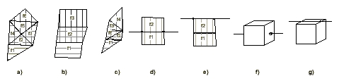
The above elaboration is under the assumption that the interior of the surface and the line have at least one node as interior. It can happen that 1) the interior of a line is exactly the link between the nodes, e.g. R403, or 2) the link between two nodes lies inside the interior of the surface. This case requires further investigation of the order in which both intersecting nodes occur in the surface boundary (see Figure 6-13d and Figure 6-13e). If they are sequential, the two interiors do not intersect. An identical problem may occur for groups of relations 6, 7, 13, 15 and 16. These are all the groups that have non-empty intersections between the interior of the line and interior of the surface, and the boundaries of the line is a subsets of the boundary or the exterior of the surface. Therefore, the test for sequential nodes always has to be performed when the interior of the surface does not contain nodes.
Existence of arcs in such cases helps to identify interior intersection (the arc will be detected as interior of the line), but the comparison of nodes cannot be avoided. All the relations that require the test of boundary intersections need operations between nodes, i.e. the same groups 6, 7, 13, 15 and 16. Therefore, it is likely to make a precise assessment without implementing and contrasting of algorithms. The important conclusion for the objectives of the thesis is the successful completion of all the relations of this configuration.
Body and line
A node or sequence of nodes is the only possible intersection
between body and line and therefore the body's interior and boundary has
to be expressed as sets of nodes. In principle, the operations needed to
identify particular relations are similar to those explained already for
surface and line. Therefore only two groups of relations, i.e. group 8
and group 14 will be discussed in detail (see Appendix
3 and Figure
6-8).
Group 8: R252, R253 and R255
The group of relations requires non-empty intersections
for![]() ,
,![]() and
and ![]() .
Suppose A is a line object and B is a body object in the relation, it is
sufficient to test the intersections
.
Suppose A is a line object and B is a body object in the relation, it is
sufficient to test the intersections ![]() and
and ![]() .
The positive (non-empty) result is sufficient to clarify the group. Next,
the exterior intersections have to be examined. The external intersection
E13 of relation R252 requires the closure of A to be a subset of the B's
closure. For this particular relation, A's boundary must be a subset of
B's interior. Finally, A's interior must be a subset of B's closure, i.e.
.
The positive (non-empty) result is sufficient to clarify the group. Next,
the exterior intersections have to be examined. The external intersection
E13 of relation R252 requires the closure of A to be a subset of the B's
closure. For this particular relation, A's boundary must be a subset of
B's interior. Finally, A's interior must be a subset of B's closure, i.e. ![]() .
The relation R253 has E14 as an external intersection, which restricts
only the boundary inside the interior of B. Hence, after ensuring that
the second boundary node is inside the interior, the condition
.
The relation R253 has E14 as an external intersection, which restricts
only the boundary inside the interior of B. Hence, after ensuring that
the second boundary node is inside the interior, the condition ![]() has
to be proved. The last relation R255 has the less restrictive E16 exterior
intersection, which requires one of the boundaries of the line to be disjoint
of B's closure, i.e.
has
to be proved. The last relation R255 has the less restrictive E16 exterior
intersection, which requires one of the boundaries of the line to be disjoint
of B's closure, i.e. ![]() .
.
Group 14: R444, R445 and R447
The relations identify configurations of spatial objects
(line A and body B) with intersecting interiors (![]() ),
boundaries (
),
boundaries (![]() ) and interior and
boundary (
) and interior and
boundary (![]() ). The relations are
appropriate examples of the same doubtful intersection as the one described
for surfaces, i.e. the interior of the body intersects with the link between
two nodes in a line (R445 and R447). The configuration of a body and a
line that corresponds to relation R444 may be such that the interior of
the line does not contain nodes. Then the intersection between the interiors
). The relations are
appropriate examples of the same doubtful intersection as the one described
for surfaces, i.e. the interior of the body intersects with the link between
two nodes in a line (R445 and R447). The configuration of a body and a
line that corresponds to relation R444 may be such that the interior of
the line does not contain nodes. Then the intersection between the interiors ![]() will
be the empty set. A solution to such exceptional cases could be an additional
operation to examine the belonging of the two "suspicious" nodes to faces
(see Figure
6-13 f,g). If the faces are different, most probably the link (interior)
between them is inside the body. The extra examination always has to be
performed when the body's interior lacks of nodes. The groups of relations
10 and 14 require the test as to the belonging of a node to a face.
will
be the empty set. A solution to such exceptional cases could be an additional
operation to examine the belonging of the two "suspicious" nodes to faces
(see Figure
6-13 f,g). If the faces are different, most probably the link (interior)
between them is inside the body. The extra examination always has to be
performed when the body's interior lacks of nodes. The groups of relations
10 and 14 require the test as to the belonging of a node to a face.
The relations considered so far are identified on the basis of the set operations (union, intersection and difference) on nodes, which will be referred to as node operations. Since the dimension of at least one of the spatial objects in the pair of geometric objects is less than 2, the only possible intersection is either a node or a set of nodes. In general, the sequence of nodes in the geometric objects is either explicitly specified (lines) or can be obtained (surfaces). Therefore, the order of the nodes in the intersection set can be established as well. Further analysis of the nodes in the intersection set may be utilised to enlarge the range of the possible relations beyond the topologically equivalent configurations. This possibility, however, is not elaborated in this text. Thus, we formulate the following general steps to categorise relations applying node operations:
6.2.3 Surface
relations
The next relations refer objects that can have a face
as a resulting set intersection. Since the face is a CnsO with a
unique shape and position, it can be employed to detect relations. The
operations operating with faces are considered face operations.
According to the definition, the closure of faces constructs the closure
of surfaces. The boundary of the surface, however, is a set of nodes. This
implies that some faces have parts in the interior and boundary of surfaces.
In this respect, the face differs from the node, which is either part of
the interior or part of the boundary. Hence, an equality of faces ensures
1) the intersection of interiors, i.e. ![]() or
(and) 2) the intersection of interiors and boundaries, i.e.
or
(and) 2) the intersection of interiors and boundaries, i.e.![]() or
or ![]() .
The second intersections have to be further clarified by node operations.
Intuitively, the question about the utilisation of only node operations
arises. Analysis of possible surfaces, however, reveals that node operations
are not sufficient. According to the spatial model, the interior of a face
can become equal to the interior of a surface (see Chapter
5), which, in practice, leads to an interior without nodes. Quite often
a surface can have all the nodes situated on the boundary despite the many
composing faces. For example, the triangulation of a complex surface always
results in a surface without nodes in its interior (see Figure
6-13 a,c). The identification of relations in these cases cannot rely
on set operations upon nodes.
.
The second intersections have to be further clarified by node operations.
Intuitively, the question about the utilisation of only node operations
arises. Analysis of possible surfaces, however, reveals that node operations
are not sufficient. According to the spatial model, the interior of a face
can become equal to the interior of a surface (see Chapter
5), which, in practice, leads to an interior without nodes. Quite often
a surface can have all the nodes situated on the boundary despite the many
composing faces. For example, the triangulation of a complex surface always
results in a surface without nodes in its interior (see Figure
6-13 a,c). The identification of relations in these cases cannot rely
on set operations upon nodes.
To illustrate the operations needed, we will start with the relations between surface and surface in IR2 because they perform with lower complexity compared to the others. The number of possible binary relations is eight as the relations (except one, i.e. R255) are the same as the relation between line and line in IR . The relation determines which topological primitives of the surfaces have to be composed initially. The interior and closure has to be available in both representations, i.e. sets of faces and sets of nodes, in order to detect most of the relations.
R031 (A disjoint B)
The relations can be identified by comparing that belong to the closure of A and the closure of B, i.e.
if ![]() and
and ![]() ,
,
then![]() .
.
The set operations union and intersection are performed on sets of faces.
R179, R220 (A inside B, B contains A)
The second relation already needs a combination of face and node operations. The first step is a comparison of interiors, for which the equality of faces is sufficient, i.e.
if ![]() and
and![]() ,
,
then![]() ,
,
for some![]() and
and![]() .
.
A supplementary step must clarify whether the common face have a common boundary with the surface, i.e.
if Fc is the common face,![]() and
and![]() ,
,
then![]() .
.
R287 (A meet B)
The relation requires analysis of boundaries, i.e. one or more of bounding nodes of A has be equal to one of the bounding nodes of B. No other common topological primitives are allowed, which can be by a test for face equality, i.e.
if ![]() and
and ![]() ,
,
then![]() .
.
The result will not change if the steps are executed in reverse order, which is more appropriate for the unification of the procedure (see below).
R400 (A equal B)
The relation can be detected by comparing the closure of surfaces and hence applying face operations, i.e.
if![]() and
and![]() ,
,
then![]() , where
, where![]() .
.
R435, R476 (A covers B, B coveredBy A)
The relation R435 can be identified by 1) test for equality
of faces and 2) test for equality of nodes. In the case of common face,
one intersection of topological primitives is non-empty, i.e. ![]() ,
and two may or may not be non-empty
,
and two may or may not be non-empty![]() and
and![]() .
The needed non-empty intersection of boundaries, i.e.
.
The needed non-empty intersection of boundaries, i.e. ![]() has
to be detected by node operations. At least one node of the nodes part
of A's and B's boundary has to be equal, i.e.
has
to be detected by node operations. At least one node of the nodes part
of A's and B's boundary has to be equal, i.e.
if![]() and
and![]() ,
,
then![]() ,
,
for some![]() and
and![]() ,
where
,
where![]() and
and![]() .
.
The non-empty boundary and the boundary intersection,
i.e. ![]() , ensures that A's
interior exactly intersects with B's boundary, i.e.
, ensures that A's
interior exactly intersects with B's boundary, i.e. ![]() .
.
R511 (A overlap B)
Since A and B overlap, the interior of both surfaces must contain at least one common face, otherwise the relation is not possible. A second node operation has to analyse the equality of boundaries, i.e.
if![]() and
and![]() ,
,
then![]() and
and ![]() .
.
The operations involved in the detection of the above relations are a combination of both face and node operations. The face operations detect the interior and interior intersection and the node operations clarify interior and boundary intersections. Compared with the same group of relations obtained for line, the complexity of operations is not higher. For example, R435 for surfaces requires one face (intersection) and one node (intersection) operations, while R435 for lines requires three node operations (two intersections and one difference). The simpler boundaries of lines (only two nodes) compensate line and line relations for the extra operations. However, this is not the case for surface and surface in IR 3.
Surface and surface relations in IR 3 are the most complex relations to identify as well as the most frequently observed in reality. The complexity of operations is a result of two factors:
Group 4: R117, R125 and R127
The first group of relations cannot have face intersections; therefore, all the topological primitives can be expressed as sets of nodes and inspection of intersection to be completed by node operations. The three relations differ in the exterior intersections E6, E14 and E16. In this case, the distinction between the intersections will be on the basis of the E6.1 (B's boundary is a subset of A's interior) and E14.1. This to say that the operations to identify this group of relations are completely equal to the ones shown for line and line.
Group 7: R220, R221 and R223
The group is an example of configurations that may result in face intersections. The first operation must be the face operation, i.e. test for equality of faces. The positive result will ensure that the interiors intersect (if all the faces of A are part of B, then the relation R220 is the candidate relation). If the test is negative, there is still a possibility for node intersections of interiors. The two surfaces may intersect in a node or a sequence of two or more nodes (see Figure 6-7). This means that a test for equal nodes that are a part of the interior is compulsory.
The next operations for this group are related to the boundaries of the surfaces, which require node operations.
R220 was already discussed above.
R221 requires two more operations (result of E13 exterior intersection). First, B's boundary must not have non-empty intersection with A's closure, i.e.
if ![]() and
and ![]() ,
,
then ![]() .
.
The second operation is needed to complete the requirements of exterior intersection (i.e. E14). The boundary of A must be a subset of B's interior.
R223 requires again two operations (based on E16 exterior intersection): 1) B's boundary must be disjoint from A's closure and 2) A's boundary (interior) must not be a subset of B's interior. The first operation is a node intersection, the second one can be completed by a test of faces (interior) or nodes (boundary).
This group of relations has demonstrated the complex examination of interior intersections. However, the complexity is even higher. If the interior of one or two surfaces do not contain nodes, e.g. the geometric interpretation for R223, A's interior and B's interior does not have a common node. The comparison of equal interior nodes must be modified to the comparison of equal boundary nodes. The order of the nodes in the surface with problematic interior must not be sequential, otherwise the nodes are part of the boundary and the relation is different. The advantage of arc maintenance in such cases is apparent. If the arc between the two nodes is defined, A's and B's interiors will have an arc as an interior intersection and hence no further operations are required. Relations R383 and R447 are examples of two extreme cases, i.e. both surfaces intersect in a sequence of nodes (two nodes) and none of the nodes is in the interior of the surfaces. However, it should not be forgotten that these cases are conditional. Additional operations are necessary only if the interior does not contain nodes.
The following generalised steps represent the identification of surface and surface relations:
Body and body
The relations between simple bodies in IR 3
supported by SSM are all the 8 obtained from eight the 9-intersection model.
The operations needed to identify the relations are briefly mentioned below
(see also Appendix 3 and Figure
6-6).
R031 (A disjoint B)
The easiest way to identify the relations is by comparison with intersection of boundaries, i.e.
if ![]() and
and ![]() ,
,
then ![]() .
.
R179, R220 (A inside B, B contains A)
First, B's interior (set of faces) and A's boundary has to be defined. B's interior cannot be a set of nodes and a set of one face because the two interiors may intersect only in a set of faces. Consequently, the identification of the relations can be simplified as follows: 1) the interior as a set of nodes must not be created and 2) at least a set of three faces has to be detected, otherwise it can be concluded straightaway that the relation is not possible.
Second, the boundary of A must be a subset of B's interior![]() ,
i.e.
,
i.e.
if ![]() and
and ![]() ,
,
then ![]() .
.
R511 (A overlap B)
In contrast to similar configurations of lower dimension, the composition of B's interior (set of faces nodes) and A's interior (a set of faces) is sufficient here. Analysis of the sets of faces for equality is the finalising operation, i.e.
if ![]() and
and ![]() ,
,
then ![]() ,
where
,
where ![]() .
.
R287 (A meet B)
Since the set intersection can be a set of faces or nodes, the boundaries of the two objects have to be available in both the set of faces and the set of nodes. The two boundary sets (expressed by faces) have to be tested for equality and if the result is the empty set, then the procedure must continue with testing for equality of nodes. It may occur that the number of nodes is more than two, which indicates a possibility for interior intersections. Hence, both the interiors must be examined for non-empty intersection.
The relation illustrates the benefits of omitting the arcs from the spatial model. The completion of relation requires boundaries of bodies to be expressed as faces, arcs and nodes. If the intersection of the boundaries is a single node, it can be detected by a third operation after face and arc operations.
R400 (A equal B)
The relation requires only boundaries of the two sets to be composed. The comparison between both the boundaries is pure face operation, i.e.
if ![]() and
and ![]() ,
,
then ![]() ,
where
,
where ![]() .
.
R435, R476 (A covers B, B coveredBy A)
The relations need the availability of boundaries and
interiors of the two objects. The interior of the covering object must
contain at least three faces, otherwise the relation is impossible. The
second step must ensure that ![]() because
the faces inside A may have common boundaries with B. The third step leads
to the same complications as above, i.e. the intersection of boundaries
must be checked with respect to faces and nodes (if the face test fails).
because
the faces inside A may have common boundaries with B. The third step leads
to the same complications as above, i.e. the intersection of boundaries
must be checked with respect to faces and nodes (if the face test fails).
Body and surface
Relations between body and surface slightly differ from
body to body. The boundary of a surface is a set of nodes, while the boundary
of a body is a set of faces. The dimension of the boundaries influences
the set intersections. The intersection of interiors![]() can
be only a face or set of faces. The intersection of boundaries
can
be only a face or set of faces. The intersection of boundaries ![]() may
result in a node or set of nodes. The intersections between interiors and
boundaries
may
result in a node or set of nodes. The intersections between interiors and
boundaries ![]() and
and ![]() can
be only a set of nodes. The relations of group 14, which needed extra testing
for line and body configuration, will be used to illustrate the operations
required (see Appendix 3 and Figure
6-9).
can
be only a set of nodes. The relations of group 14, which needed extra testing
for line and body configuration, will be used to illustrate the operations
required (see Appendix 3 and Figure
6-9).
Group 14: R444, R445 and R447
Whilst the interior of the body is sufficient to be represented
by a set of faces, the boundary of the body and the interior of the surface
has to be expressed by a set of faces and a set of nodes. Under these considerations,
the identification of intersecting 1) interiors (![]() )
is a face operation, 2) boundaries (
)
is a face operation, 2) boundaries (![]() )
is a node operation and 3) interior and boundary (
)
is a node operation and 3) interior and boundary (![]() )
is a face operation. The interior intersections are easy to clarify because
they are based on face operations. The external intersection of R44 is
E13, which implies that the interior of the surface is a subset of both
interior and boundary of the body, i.e.
)
is a face operation. The interior intersections are easy to clarify because
they are based on face operations. The external intersection of R44 is
E13, which implies that the interior of the surface is a subset of both
interior and boundary of the body, i.e.
if ![]() ,
, ![]() and
and ![]() ,
,
then ![]() .
.
The completion of this operation ensures that the boundary of A is also a part of B's closure. R445 has exterior intersection E14, which allows a part of the interior to be outside the closure of B; however, the boundary must be a part. Therefore, the boundary of A has to be surely a subset of B's boundary, i.e.
if![]() and
and ![]() ,
,
then ![]() .
.
R447 means that a part of the boundary and the interior of A are outside the closure. It is easy to conclude that in that case a face operation to test the interior of A and closure of B is sufficient, i.e.
if ![]() and
and ![]() ,
,
then ![]() .
.
In contrast to line and body configuration, the relations of group 14 can be identified easier. The remaining relations possible for body and surface do not require any specific considerations different from the ones discussed above.
6.3
Usefulness of the decimal codes
The discussion on operations given above reveals interesting
properties of the relations based upon the decimal codes, i.e.:
Another significant advantage of the codes is their utilisation to name the relations. The introduction of names for all the 69 relations between different objects is a difficult, hardly realistic task. The names given to the eight relations already create an ambiguity. As was shown, the relation overlap between lines is not the same as the overlap relation between bodies (see Figure 6-2 and Figure 6-6). Usually, the names established for relations so far are on the basis of observations of the geometric configuration. While it is quite easy to create a clear perception about, e.g. a parcel, which meets a street in 2D space, it is much more difficult to judge the configurations in 3D space. The same relations may look different due to 1) different dimensions and 2) topological equivalence. For example, all the surface configurations, which are presented as relations with codes from R063 to R159 and from R221 to R383 might be interpreted as meet interaction (see Figure 6-7). However, the bodies' configurations for relations R253 and R255 can hardly be identified as meet (see Figure 6-8); most probably one would say that the line is partially inside the body. The topologically equivalent relations between surfaces, denoted as R233 (see Figure 6-10), create different perceptions, i.e. they cannot be unified under one name. For example, R233 b), c) and h) case may be considered meet, while the rest of the cases can be classified as intersect. In this respect, the code, being a decimal representation of the exact sequence of binary intersections needed for a relation, is not dependent on human perceptions or the dimensions of objects. Giving a unique notation of a relation, it can be used as a standard manner to name relations regardless of auxiliary considerations.
6.4 SSM for spatial analysis in urban areas
Chapter 3 has clarified a generic set of spatial relationships that has to be supported by the GIS model. The demanded relations were denoted as adjacency, inclusion, part-of and direction (e.g. above, under). The relationships which can be obtained employing the 3D topological relations discussed above are adjacency, part-of and inclusion. Spatial relationships related to direction can be detected only by metric computation on the basis of either object's CnsO (i.e. nodes) or co-ordinates of maximum bounding boxes of a 3D R-tree (see Chapter 7 and Chapter 8).
Practically, the scope of relationships, which can be detected by SSM is far beyond the demanded relations. For example, the user can translate the topological relations of groups 2,3,4,9 and 10 (see Appendix 3, Table 1) as adjacency. Some of the relations of groups 6,7,8,14,15 and 16 might be related to inside/outside relationships, others to the relationship part-of. Apparently the issue needs further refinement with the user.
Moreover, some of the possible relations may never be needed in reality. The possible spatial relationships between some objects may be very limited. For example, the relationships between two walls or rooms are most likely to be only meet or disjoint. The relationship between a window and a wall is either disjoint or inside or meet or (eventually) equal. This is to say that the semantic characteristics ("meaning") of the object may be used to further facilitate development of operations. Consequently, the development of relationship operations is dependent on the spatial objects maintained. This implies that the needed operations have to be clarified with the user after the specification of the objects.
The spatial relationships are the selection criteria of the relationship operations (see Chapter 2). Ensuring support of spatial relationships, SSM enables a large group of spatial queries and analysis to be performed.
It was demonstrated that the possible binary relations according to the 9-intersection model can be identified with the data organisation proposed in SSM. The possible relations are derived for simple objects, i.e. lines with two disconnected boundaries, surfaces without holes and bodies without tunnels.
The estimation of the suitability of SSM to perform spatial analysis is based upon a particular category of queries. The assumption is that a specific relation has to be identified between two known objects. Queries that require such an approach can be "examine whether the relation between the two roofs is R287", "find the building adjacent to the street ", "check whether the pipe goes through the room", "is the tree outside the parcel?", "find the shortest way to the station". In the last example, the answer cannot be obtained by identifying a single topological relation; however, it can be derived by analysis of several sub-queries, each of which is the relation meet between surface and surface (streets). The dimension of the objects and the code of the relation are known in advance. The expected result is either positive (yes, the relation between the objects is the required one) or negative (no, the relations between the objects is different). The case is the easiest for analysis and implementation. The sequence of operations can be selected appropriately to optimise the query.
In reality, two more categories of queries are possible. The first one requires recognition of the relation between two objects. This is to say that the dimension of the objects is known but the code of the relation is unknown. For example, "what is the relation between the house and the garage", "find the type of interaction of the railway and the road", "what is the relation between the parcel and the lamppost". Such queries, most likely, will require the examination of both closure and exterior intersection between topological primitives. If the objects are of dimensions 2 and 3, then the boundaries and interiors have to be inspected for both face and node intersections. Indeed, if the result of the closure intersections places the relation in a group, where the inspected configuration of objects cannot have another relation, then the examination of the exterior intersections can be omitted.
The second category of queries refers to the identification of a relation regardless of the dimension of objects. An examples of such queries are "find all the objects, which meet", "find all the common walls in the neighbourhood". The query is relevant for a consistency check in the object reconstruction phase. An implementation of the query is given in Chapter 7 in two ways, i.e. "find objects with common nodes" and "find objects with common faces".
As was shown, the operations needed to complete inspection of any relation are from the set operations, i.e. union, intersection and difference. Some exceptional cases require testing for a sequential order of nodes and belonging to a face. Since the node and the face are sets, the test for belonging can be converted to the operation intersection. The sequential order of the nodes in a face is explicitly specified (see Chapter 5), which allows the two sets, i.e. 1) the set intersection and 2) the set of nodes in a face, to be compared as ordered sets. Thus, the identification of topological relations relies entirely on the standard set operations. The benefit of this conclusion is that the operations are compatible with the standard SQL operations select and join, which is a premise for an effortless implementation in RDBMS.
The omission of arcs in the spatial model does not disturb the recognition of topological relations. Two problematic cases concerning inspection of interiors require more operations. Both cases regard the relations between lines and surfaces or bodies. The intersection between the two interiors might be "empty" of nodes. Additional tests have to be completed to inspect whether the link between two nodes of the line is exactly inside the interior of the surface or the body.
The maintenance of less CnsO exhibits advantages in several ways. The topological primitives have to be presented only as sets of nodes (for operations between points, lines, surfaces and bodies) and sets of faces (bodies) and combinations of them (surfaces and bodies). The intersections between the objects are interpreted as a set of nodes or a set of faces. The operations needed for manipulations of objects are only node and face operations. The maintenance of arcs will require a presentation of the topological primitives by nodes, arcs and faces. In many cases, it is hard to predict the dimension of the intersection between two objects, which may need a test of all the constructive objects. The test for arcs is advantageous for the exceptional cases mentioned above and disadvantageous for the remaining ones. Hence, if the exceptions are more than the regular cases, some efficiency can be expected in the identification of body and surface relations (i.e. the test could be completed by faces and arcs). Operations with lines always require node operations due to the disconnected boundary of the line. This means that the topological primitives have to be expressed by the three constructive objects. This already means an increase in the number of operations, to significantly more that the required for resolving the ambiguous combinations of interiors without nodes. Therefore, we expect better performance in the completion of spatial analysis from SSM than from a spatial model maintaining arcs. Chapter 8, Case study 3 presents a comparison between 3D FDS and SSM that proves the expectation for the group of spatial queries implemented.
Our study considers only simple objects. To model and
analyse the real world, however, simple objects may not be sufficient.
For example, a wall of a building with windows or a roof of a building
with a complex facet construction may need to be represented as surfaces
with holes. SSM requires such surfaces to be defined as complex objects
(see Chapter 5). The binary relations between
complex objects require further investigations in three directions: 1)
definitions of rules to compose complex objects, 2) definitions of the
topological primitives and 3) derivations of binary relations between complex
3D objects. Some of these issues are already discussed in the literature.
Mechanisms to identify binary topological relations between surfaces with
holes in 2D space are reported by Egenhofer et al 1994. Hornsby and Egenhofer
1998 explore some operations on composite objects with respect to the different
rules they are created. Egenhofer 1994 and Gapp 1994 present a formalism
to derive knowledge about the composition of two binary relations over
a common object.