- Figure
8-1: Free SQL query (see SGI script) Figure
8-2: Specialised HTML forms
 |
 |
The chapter is organised in four parts, i.e. a description
of the prototype system and three case studies. It starts with a short
overview of the components used for the client/server implementation, i.e.
Web server, DBMS, Web and VR browsers, Perl language, and motivates the
selection made. Case
study 1 discusses the GUI and several examples of basic semantic and
spatial queries and the corresponding visualisation of results. Case
study 2 discusses the building of the 3D R-tree. Case
study 3 discusses the selected representative queries used to evaluate
the performance of SSS. The experiments are performed on the two test sites
discussed in Chapter 7. A final discussion
of the results obtained concludes this chapter.
8.2.1 Data query8.3 Case study 2: Dynamic creation of LODExample 1: Query of spatial and attribute information per object (pull-down menus)8.2.2 Data visualisation
Example 2: SQL queries: "SELECT" and "SELECT+visualise"
Example 3: Common faces
Example 4: Visibility check
8.2.3 Data modificationExample 5: Modification of information8.2.4 Data exploration and manipulation
8.3.1 3D R-tree creation8.4 Case study 3: Performance
8.3.2 Organisation of LOD
8.3.3 Dynamic creation of LOD
8.4.1 Size performance8.5 Summary
8.4.2 Time performance
The components of the proposed system architecture (recall Chapter 4, Figure 4-7) are a Web server, RDBMS and language for CGI scripting (on the server site), VR and Web browsers (on the client site) and corresponding hardware. The components were selected in accordance to the fundamental consideration for a low-cost and easy-to-implementation solution. In general, proof-of-concept system architecture inquires minimal investments and a possible realisation in a relatively short time. A more pragmatic aspect the low-cost components will be of practical benefit for the intended application of the system architecture, i.e. municipal activities and service. Therefore the study and selection of components was limited to the software and hardware currently available in ITC, freeware modules and evaluation versions of commercial software. A short overview of the important features motivating the choice is presented below.
Apache is the Web server selected for the prototype system. The Apache server is a freely available server written by a non-profit team of developers, i.e. the Apache software foundation (see Apache 1999). Officially released as Apache in April 1995, the daemon was already the most popular one on the Web based on HTTP protocol. Since that time, it has gained a lot of popularity with its stable work, many advanced features and a relatively easy set-up (see Stein 1997). Apache works under many operation systems (Windows, UNIX, Linux) on different hardware platforms (i.e. microcomputers and workstations). The requirements for available disk space (1.5Mb), processor (486DX) and memory (16Mb RAM) are moderate. The server has already been in use quite a long time and most of the software problems have already been resolved. All these considerations motivated the election of the Apache server. Some alternatives are the commercial Web servers WebSite (see O'Reilly and Associates 1999), WebSTAR (see StarNine 1999) and Microsoft®SiteServer (see Microsoft 1999). WebSite runs under Windows operation system (Windows95 and WindowsNT). Some initial experiments were carried out within the one-month evaluation period provided by the demonstration version. The server has quite similar features to Apache. WebSTAR is a Web server for Machintosh. Microsoft®SiteServer runs only under WindowsNT with the suite of Microsoft products, e.g. Visual C++ and Microsoft Foundation Classes (MFC), Java++, Microsoft SQL server, ODBS, etc.
MySQL is a client/server relational database management system implementing SQL. MySQL consists of a server and client programs and libraries. The freeware server was launched for the first time in 1996, with the intention of dealing with very large databases, which no vendor can provide. The developers (see TcX, DataKonsultAB, 1999) provide numbers of manageable tables and records, which are compatible with about 100 Gb data. Despite some limited functionality (hosted SELECTs and view are still missing), the database system is widely used for a variety of applications. It is available for almost all kinds of hardware platforms and operation systems. A variety of Application Programming Interfaces (API) in different languages (C, C++, Perl, Python, Java, TCL) are freely available on the Web. Other attractive features are: a very fast JOIN operation, the possibility to access tables from different databases in the same query, a very fast B-tree indexing based on disk tables and compression, etc. Some benchmarks have showed significantly better speed performance compared with other DBMS (mSQL, PostgreSQL, Microsoft Access, Oracle). The database does not provide a GUI, e.g. "query by example", which, however, was not needed for the system architecture. Another freeware DBMS are mSQL (see Hughes Technologies 1999 and PostgreSQL (see PostgreSQL, Inc. 1999). MSQL is a very light database system designed to provide fast access to small data sets. Since interest in the database is increasing, the last release promises an enhanced functionality. PostgreSQL is an object-oriented (OO) RDBMS.
It supports SQL3 and provides extended OO possibilities to define types and classes. The database system is available for Unix-like operation systems. At the time of development of our prototype system, the performance of PostgeSQL (Postgres95) was worse than MySQL and the availability of APIs was rather limited. These features are considerably improved in the new releases, which makes PostgreSQL an option for a DBMS in our approach. Some initial tests (mostly spatial queries in 3D FDS and SSS) carried out with Microsoft Access have shown rather unsatisfactory performance, which eliminated the RDBMS on a very early stage.
Perl was the language used in our system to write CGI scripts. In general, CGI scripts can be created in any programming language (C, C++, Python, Java, TCL, Pascal, Delphi). The compiled languages such as C and Pascal gain in speed in the case of computational operations. The interpreter languages (Perl, Python, TCL), are more suitable when command-line-based operations have to be performed. A typical example of such operations is the submission of SQL queries to a database. Developed originally as a Unix language, Perl is now available for most of the computer platforms and can be freely downloaded from Comprehensive Perl Archive Network (see CPAN 1999). Another crucial feature of the language is the large number of freeware CGI scripts, libraries and APIs, which, further extended, save a lot of programming effort. Two of them, i.e. CGI.pm and DBI.pm to create fill-out forms and access MySQL database, were used for the implementation of the system. More information about them can be found in Bunce 1999, Stein 1998 and Wiedmann 1998.
The Web server and the RDBMS were installed under LINUX on Pentuim 133 MHz, 96 Mb RAM. The tests were conducted from a client station equipped with the Web browser Netscape (see Netscape Communication Corporation 1999) and the VR plug-in Cosmo player, running under Windows 95. The user on the client site can use any other Web browser supporting frames, e.g. Microsoft Explorer, and any VR browser (supporting VRML2.0), which has a plug-in version for the selected Web browser (see Web3D Consortium, 1999)
In general, different suites of components can be realised under the condition of a low-cost system. Some examples are listed below. The current configuration, i.e. Apache, MySQL and Perl, can be installed under Windows 95/NT or any other UNIX operation system. Apache server and Perl language can be combined with mSQL (for small data sets). Apache server, PostgreSQL and Python scripting language are yet another possible configuration for UNIX (LINUX) operations systems. API written in Python to access PostgreSQL is already available. This configuration premises the ability to compose complex object types at database level and perform extended SQL queries, features which may facilitate and simplify the CGI scripting. In principle, Apache server can be integrated with Microsoft Access DBMS, but the scripting language has to be changed to C or Pascal (Delphi). Ingredients for our system architecture can be selected from among commercially available systems as well. Practically any DBMS (Oracle, Informix, SyBase, DB2, etc.) can be employed for a data warehouse. The scripting language in most of the cases has to be C or Pascal.
The hardware configuration selected as a server is moderate. The understanding was that an acceptable performance on such equipment with test data would be a premise for a good performance on a better hardware configuration with larger data sets.
The prototype system is used to verify three concepts proposed in this thesis. First, it has to demonstrate that the approach for access and visualisation of 3D GIS data is feasible. The ways to specify queries and explore results, discussed in Chapter 4, are illustrated by an experimental GUI elaborated in Case study 1. Second, the prototype system has to provide evidence of an improved performance of SSS. A set of representative queries on two data sets are used as an indicator. The type of the queries and the approach to testing the results are explained in Case study 3. Finally, the prototype system has to validate the R-tree indexing in two of its aspects: 1) the spatial grouping of objects is appropriate for dynamic creation of LOD and 2) the code introduced in Chapter 7 is efficient. For this purpose, an algorithm for the R-tree construction, applying different constraints, is presented in Case study 2. The effect of R-tree codes with respect to the asseveration of the database traverse is then discussed in Case study 3.
All the tests are performed on the two experimental sites
created in the Chapter 7. The first test site,
i.e. the central part of Enschede, contains photo-textured buildings and
terrain, trees, lampposts, streets and parking lots. The model is relatively
small but contains most of the relational tables according to SSS. The
second test site, i.e. Vienna, consists of only buildings. The test site
is simpler in terms of a variety of objects and object components (only
the BODY_G, BODY_T and BODY_A are created); however, the number of objects
is quite high. The first data set was used mostly to illustrate the GUI
and suggested manner to compose queries, extract data and perform results.
The second one was employed in regard to speed performance of the system.
The case study on dynamic LOD creation presents examples from both data
sets.
8.2
Case study 1: GUI for query and visualisation
The GUI presented is organised in framed HTML documents in maximum two windows. According to our approach, the HTML documents are intended for the formulation of queries (typing or selecting parameters) and to display information (text, raster, movie, sound, etc.). Basically, the Web browser can visualise every file format that has defined MIME format and corresponding plug-in or helper applications assigned to it (and is available on the client site). The list of standard formats is already quite long and can be additionally extended (see Stein 1997). The VRML document is used to provide a graphical display of 3D spatial analysis and to facilitate the identification (by visual observation) and selection of objects to query. Here, we illustrate four of the steps presented in Chapter 4, i.e. query, data visualisation, data modification and local query (see also Zlatanova 1999a, Zlatanova 1999b). The first step, i.e. user identification and database selection is of a minor significance for the evaluation of system functionality and therefore is not implemented.
8.2.1 Data query
The development of GUI was guided by the investigations
into user requirements. Chapter 3 has already
discussed the variety of users approaching the municipal 3D GIS and their
probably different experience with GIS. In this respect, the GUI has to
allow an easy, intuitive way to query a broad spectrum of spatial and semantic
information (see also Coomans et al 1997). Therefore, we have experimented
with three conceptually different approaches to requesting for information:
multiple-choice, one-line SQL queries, formulation of complex queries.
The multiple-choice forms offer a very simple way to obtain information
about certain objects. The limited choice is the only disadvantage. We
suggest these forms be used only for query of information per object. Then
the menu may contain all the items of interest per object. Example
1 discusses the steps to obtain information and the layout of the form.
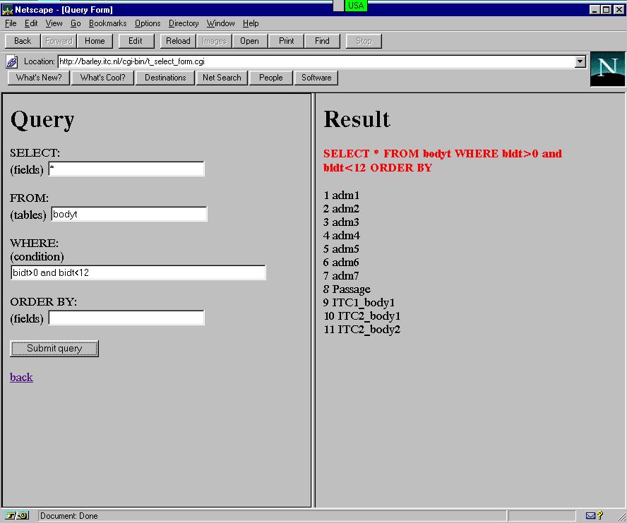
Qualified users are allowed to send SQL statements to the database. The SQL statement is specified in an HTML fill-out form. The result of the query is displayed either in an HTML or in a VRML document. Several SQL forms treating different situations, i.e. "free SQL query", "SELECT", "SELECT+ visualise " are designed and tested. The free SQL form is the simplest one: a two-section frame gives the user the possibility to type an SQL query and look at the result in the second part. In fact, the Web browser acts a standard line interface of the DBMS. Currently, the form works only with text information (see Figure 8-1). In general, most of the SQL command can be "dressed" with a GUI based on HTML fill-out forms. Depending on the desired SQL statement, the layout may vary. For example, the form "SELECT" offers a separate text field for each key word (i.e. select, from, where, order by) of the statement. Example 2 explains the forms in detail.
The forms mentioned above allow query of spatial and semantic information of objects that can be expressed by one SQL statement or selected by a multiple choice menu. A large number of queries are more complex and need a host language to process the result of series of SQL statements (see Chapter 2). We have developed several specialised HTML fill-out forms to illustrate the way we resolve these cases, i.e. Example 3 and Example 4. We group and offer all the specialised forms to the user in an individual HTML document (see Figure 8-2).
|
|
The example presents a way to extract information about a particular object, i.e. the user visually decides which object to query inside the VRML document. The user has at his disposal a two-section frame. One of the sections displays the VRML document and the other can be used for instructions. The VRML document is created in such a way to provide point-and-click operation. In the snapshot (see Figure 8-3), the building closer to the viewer is "equipped" with a VRML sensor and thus available for pointing. A click with the mouse on the building activates a CGI script, which delivers the Query-Result sections to the client station.
In the Query section a pull-down menu offers several options: co-ordinates of the building, image file used for texturing the walls of the building (in this example one image file is used for all the four textured walls), a VRML containing only the building, and the interior of the building. The choice made in the first Query section has to be sent to the server by pressing the Submit button. The CGI script processes the form and creates a new HTML document. The snapshot represents the case when the interior of the building is selected. Since the interior is kept as a panoramic movie, the newly created HTNL contains the name and the location of the file. The browser displays the delivered HTML document in the Result section of the frame. This option needs the SmoothMovie plug-in for visualisation. The snapshot of the screen is made at the final stage, i.e. the interior of the building is selected, the HTML document has arrived and the panoramic movie plug-in is activated. This example is the realisation of the two-step query discussed in Chapter 4. The first step is identification of the building and the second step is selection of the information. The query in this example is restricted to the several options in the pull-down menu. The choice, however, can be further extended by activation of a CGI script to deliver an SQL form with larger possibilities for query.
Figure
8-3: Query of spatial and semantic information about an object (see CGI
script)

Note that in the example the reference between the VRML object (a node in the VRML document) and the ID of the corresponding object in the database is already established. The ID recognition of the objects, however, has to be completed prior to the stage described in the example. Recall Chapter 4, that either each object (resp. node in VRML) has to have its own CGI script (with known ID) suitable for user request, or only those selected by the user. Bearing in mind the large number of CGI scripts in the first case, we give preferences to the second option. Unfortunately, CGI scripts do not have access to VRML nodes, cannot control their status and thus no information about the actual ID of the object is provided. This information has to be given by the user. We suggest a method of organisation by an intermediate VRML document, where the user will pick up the ID of the objects by using the extended TouchSensor, described as a new PROTO node (Chapter 4). In practice, an event "mouse-over-object" activates an ECMAscript, which visualises the ID and an event "mouse-click-on-object" activates a CGI script, which delivers an HTML fill-out form where the user can type the ID observed. Another CGI script creates dynamically the HTML frame and the VRML document described in the example above. The VRML document already contains a reference between ID and nodes for all the objects pointed by the user.
Example 2: SQL queries: "SELECT" and "SELECT+visualise"
The primary interest in this research is the visualisation of 3D spatial queries. "Translated" to our approach, this means that the CGI script not only retrieves the data from the database but also represents the result in a VRML document in an appropriate way for the user. As discussed in Chapter 4 and Chapter 5, the syntax of the VRML requires a geometric description different that maintained by the conceptual model. Therefore, the SQL statement has to ensure sufficient data for VRML creation and efficient ordering of faces. The data and the order required are displayed in the fill-out form. The interface is based on a two-section framed HTML document. The left part is reserved for typing SELECT statements and right part is used to display either HTML or VRML documents. The form correctly filled is sent to the server and a HTML document is assembled as a first document (on the left side of the frame). On the basis of the result obtained, the user decides whether to continue with VRML creation. The intermediate step is included basically to provide greater freedom on the result. It can be avoided with a control over 1) the fields in the form and 2) the data extracted from the RDBMS. Such control, however, will restrict the functionality of the form to only VRML documents. Figure 8-4 shows a snapshot of the Web browser after VRML visualisation.
Figure
8-4: SQL queries: SELECT and visualise (see CGI
script)
The free access to the database provides a mechanism to specify and display a wide range of spatial queries. Each request in the spatial domain (formulated by spatial or non-spatial restrictions) which can be described in one SELECT statement can also be visualised in a VRML document. Examples of such queries are "which is the highest building?", "show the buildings in a particular area", "show all the streets", "show all the administrative buildings". The same mechanism can be used to create DELETE, UPDATE, and INSERT forms to edit data.
This example illustrates retrieval of neighbourhood relationships, i.e. "common nodes" and "common faces". In the form, the user has to clarify the objects that have to be inspected, i.e. the user has to be aware of the objects' ID. As discussed above, the ID can be provided with a VRML document. An option to analyse the relationship between two objects is offered as well. An asterisk, instead of ID, extends the search among all the objects in the database. Figure 8-5 is a snapshot of the query "show all the common walls". The fields for ID are filled-in with asterisks. The right section of the frame displays the two bodies obtained. The invisible face between them is the common face. Since the query cannot be completed on the basis of SQL queries, the programming language used for CGI scripting (in our case Perl) acts as a host language.
Figure
8-5: Specialised queries: common faces (see CGI
script)
The last example demonstrates facilitation and simplification complex analysis by an appropriate 3D visualisation. The field of vision (or line of vision) is important information for telecommunication, geodetic, military applications, etc. For example, a mobile telephone company could be interest in verification of the actual position of a transmitter. This can be translated to a query "check the visibility between the position of the transmitter and the roof of that building" or "show the range of the transmitter". To require such information, several ways of specifying the query a possible: 1) co-ordinates of begin and end points of the line of vision, 2) ID of the two points or 3) one point and the range of view (represented as e.g. cone of view). In our example, we consider the case when the two co-ordinates are to be input. The outcome of the query must be a set of objects, which disturb the view. Theoretically, this query requires complex 3D intersection algorithms between the line of vision and the faces forming the objects in the range of the line. Here, we present a simple solution based on a visual inspection of the actual path of a traversing line between the two points. The line of vision is drawn in the VRML world and the user can observe the points of disturbance. A form to illustrate the idea is shown on Figure 8-6. The user has to type the co-ordinates of two points and as a result she/he gets a VRML document with a subset of the model surrounding the points of interest. A line through the points traverses the direction. In the VR browser, the user can navigate around the disturbing object, inspect and evaluate the situation. Appropriate sensors (extended Touchsensor presented in Chapter 4) attached to the objects provide identification information, e.g. the ID of the objects or the name of the owner (company or private person).
Figure
8-6: Specialised queries: visibility control (see CGI
script)
The visualisation of spatial data and more specifically results of 3D spatial analysis in our approach has three aspects: 1) geometric representation, i.e. objects vs. parts of objects, 2) components of the scene and 3) means for further exploration.
In this thesis, we assume that objects with a complete set of CnsO will be visualised on the screen. For example, the result of the spatial query "show the walls of buildings, which touch this street", will be represented by the street and surrounding buildings (the walls might be highlighted or not) instead of the street and the adjacent walls. Since we provide the user with the possibility to navigate inside the world, we consider the supply of "shape realism" compulsory. All the examples of VRML worlds given in the thesis are under the assumption of complete geometric representation of objects on the screen.
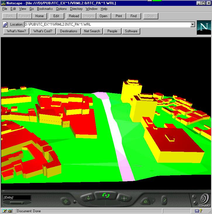
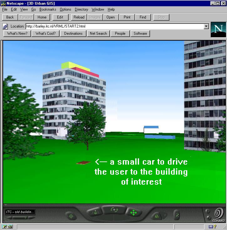
Different approaches to compose a scene in a VRML document can be implemented. The simplest way to get fast results on the screen is the visualisation only of the objects elected by the query displayed in shading mode (see Chapter 2). Some of the queries described above are examples of this approach (Example 2, Example 3, Example 4). However, very often the view with the objects is very limited and does not provide information about the surroundings. A part of the town (neighbourhood, several streets with buildings along them) commonly has to be included in the VRML document to facilitate the orientation. Techniques such as different pre-defined views, highlighting, blinking, guiding animation or selective texturing can be applied to focus the attention. The objectives of the thesis do not include detailed investigation into the problem. Figure 8-7 gives examples of a highlighted street and guided animation. The "car" (a small red parallelepiped in Figure 8-7b) brings the user to the building selected by a query. The part of the VRML document containing the VRML nodes controlling the animated car is given in Appendix 4. More examples on focusing the attention by applying VRML techniques can be found in Ogao 1997.
Since the enhanced techniques to display spatial queries and attract the attention require extra VRML nodes, they have to be used with attention. To our experience, the user has to be prompted to request for specific way for visualisation. For example, before the actual composition of the VRML document, the user can be asked to select between objects for visualisation. Such approach is followed in Example 4, i.e. prior the VRML design the user may choose whether to have DTM and grid of co-ordinates visualised. Figure 8-6 is an example of a grid selection.
a) highlighted street |
b) guiding animation |
Changes at database level can be executed either by the "free SQL" form presented earlier or by development of forms similar to "SELECT+visualise". Both ways, however, require the user to be skilled in typing SQL queries. Since this is not always the case, we have developed an alternative approach based on multiple choice and specific fields to import new values.
Example 5: Modification of information
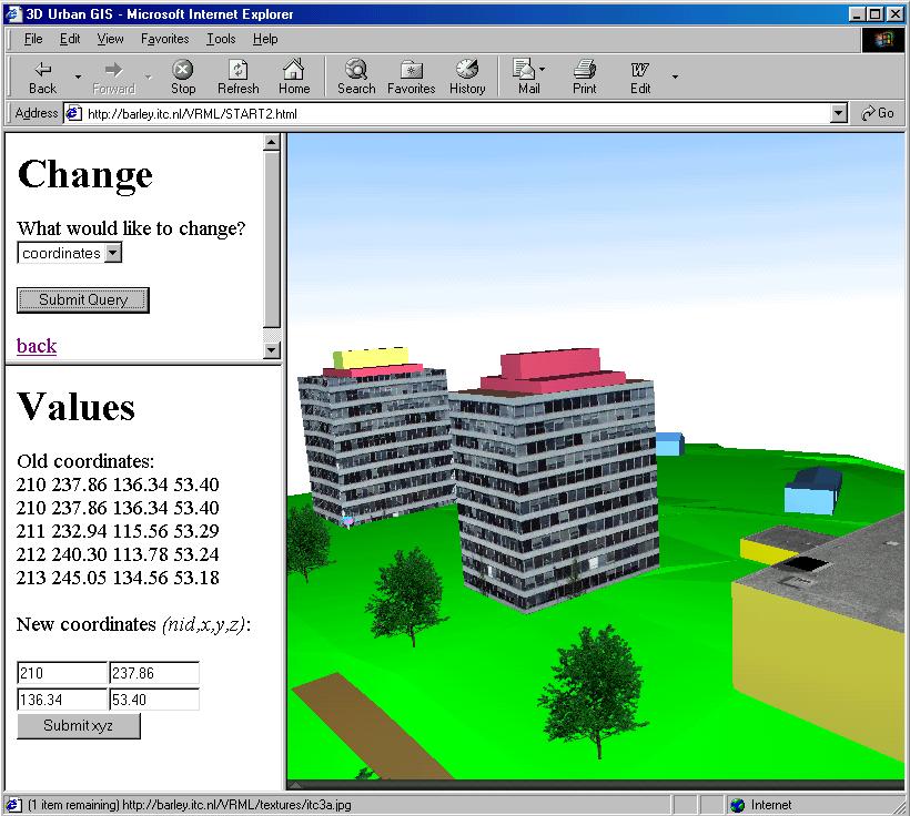
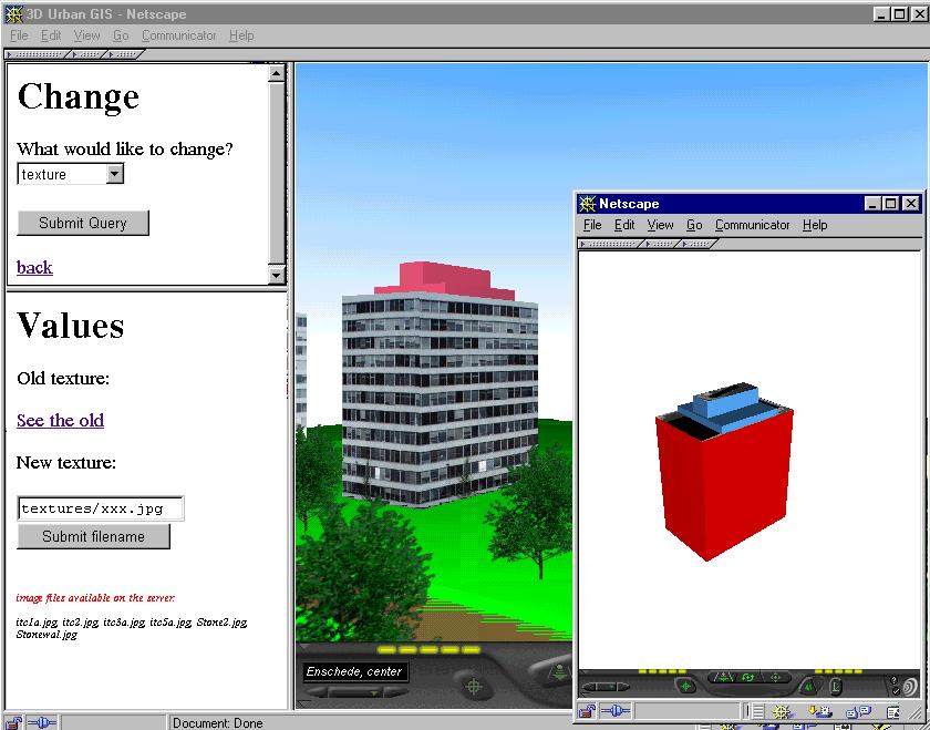
The example form suggests a method of edit operation at database level. Here, the dynamically created VRML document is used for verification. Again the initial VRML document has to be equipped with the necessary sensors to detect user actions on a particular object. A click on an object activates a CGI script, which provides two sections: a Change section where the optional changes are listed and a Values section to display the old values and introduce new ones. Currently, the form offers three options: change of co-ordinates of points, change the name of the image file used for texturing and change of the texture co-ordinates. The snapshot given in Figure 8-8 shows "change of texture co-ordinates". The operation is relevant for users who want to experience, e.g. a new façade of a building. They will need to have the name of the image with the new façade and a mechanism to reference points from the image to the real co-ordinates of the geometry of the building. The steps necessary to match texture onto the faces are listed to the left side of the snapshot (see Figure 8-8). A submission of the type of the operation (i.e. change texture co-ordinates) activates a search in the database for the old image co-ordinates. An HTML document with co-ordinates and field to type new ones is delivered in the section Values. In this section, the user has to type the new co-ordinates. The submission of the new values to the server will modify co-ordinates in the corresponding database fields and will create a VRML document for verification (i.e. VRML with results). The texture can be adjusted after several repetitions of the operation. The way to edit co-ordinates (see Figure 8-9) or change the name of the image files for texturing (see Figure 8-10) is identical to the one described for textures.
Figure 8-8: Editing co-ordinates for texture mapping of a building (see CGI script)
The local query refers to operations, which are already coded in the VRML document but the user has to activate them (see Chapter 4). To demonstrate such operations, we assume that one building has several textures stored in the database and the user needs to compare them. Then they can be included in one VRML document but only one of them can be visible at a time. We have assembled certain VRML nodes, which provide the user with means to switch them. The second textured building in the last example has a sensor attached to it (see Figure 8-8). A click on the building will result in replacement of the façade of the building, i.e. the image file used for texturing will be replaced with a new one. The difference with the previous example is that no connection to the server is made. The specific VRML nodes (sensors, routes and ECMAscript) link the "switch-on-click" operation to a script, which sequentially changes the images at every clicking on the building.
 |
 |
8.3 Case study 2: Dynamic creation of LOD
This case study is devoted to the investigation of algorithms to group the objects in 3D R-tree structure. The issue has two specific aspects, which need elaboration. First, the intended R-tree is three-dimensional and most of the algorithms focus on 2D cases. Second, with respect to the logical design, our 3D R-tree is introduced for spatial indexing and dynamic creation of LOD (see Chapter 7). As discussed in Chapter 4, the VR browser is capable of dealing with different LOD, i.e. the VR browser chooses the needed LOD and decides on the moment of switch. The LOD, however, have to be available in the VRML document. We have selected a creation of LOD based on an on-fly extraction of data from the MBB of an R-tree. This is to say that some of the MBB of the R-tree will be visualised on the screen, replacing the object's detailed geometric description. The case study investigates and selects a method for a 3D R-tree construction, which provides MBB appropriate for LOD.
The critical issue in the R-tree creation is the consolidation of objects in a leaf. The algorithms to build the classical R-tree and its modifications (e.g. R+) are based on 2D subdivision of the space with respect of the shape of the objects. Kofler 1998, investigates the only R-tree based on 3D boxes instead of triangles. Despite the third dimension, the grouping of the objects is based on a predefined subdivision of 2D space. A 2D rectangular mesh with constant width controls the grouping. One R-tree leaf contains the objects that fall in a particular patch of the mesh. Moreover, all the objects of which the upper left corner of their 2D projection falls in the same rectangle are grouped in one R-tree leaf. If the object does not fall completely in the rectangle, an enlargement of the bonding box is done to comprise the object. The minimal width of the mesh is calculated on the basis of the average object size. The method allows the construction of a very well balanced R-tree in 2D space.
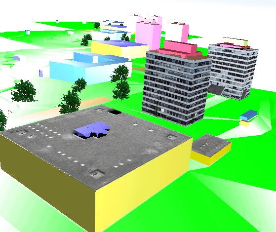
The criterion to group several objects in a leaf is usually not influenced by the third dimension when the R-tree is utilised for spatial indexing. In our case, however, certain MMB are part of the scene. They will appear behind the detailed objects and will participate in the formation of the town's silhouette. Small houses and buildings in general will have no impact. The high ones, however, are most likely to be visible. Being a part of the R-tree leaf, the building may be grouped with other buildings in a significant distance from each other. Thus the MBB for these leaves will have the height of the highest building and foundations covering a large area, e.g. one neighbourhood. The MBB displayed later as LOD will create a misleading perception of a group of high buildings in the neighbourhood.
In our approach, we investigate the impact of an object's height on the shape and size of the R-tree boxes. The intention is to group the nearest objects and preserve (as much as possible) the structure of the town until certain levels of the R-tree. For example, the parent boxes of the R-tree containing high buildings have to remain the highest box and have to be relatively situated at same location. Respectively, it has to be possible to indicate the areas with low density of houses. R-tree boxes created under such considerations can be used to select geometric descriptions for LOD.
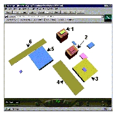
The MBB of objects is based on the traditional approximation of MBB, i.e. its faces are parallel to the x, y, z axis planes. The incorporation of an object in a node, investigated here, is based on two parameters, i.e. the number of R-tree entrances and the distance (or angle) between the objects at first step and the MBB afterwards. Three approaches to group objects were investigated: 1) horizontal distance, 2) inclined distance and 3) minimum-maximum angles between the mass centres of the objects (MBB). First and second approaches select the N-closest (N is the number of the R-tree entrances) objects among all the objects, according to respectively, the horizontal and inclined distance between mass centres. A threshold prevents incorporation of distant objects. The third algorithm selects the objects according to the height of the MBBs, i.e. two object are assigned to one parent node if the angle between the mass centres falls in a given threshold. These three approaches for grouping were tested with the Enschede data set. The results are presented in Figure 8-11. The different cases are snapshots of the MBB visualised in VRML documents. The orientation of the objects in all the snapshots is approximately the same in order to facilitate the comparison. Thus the two MBB representing the highest buildings 1 and 2 (see Figure 8-12) in the site are always at the top of the snapshot (bordered by a circle in Figure 8-11 1).
Figure 8-11: MBB of objects: different criteria for grouping (1, 2, 3, 4, 5, 6, 7, 8, 9, 10, 11 and 12 in VRML)
 |
 |
Variations on the basis of the distance/angle criterion are less apparent. The case 9) N=4, A indicates that the usage of only the angle criterion may lead to very large box composites. In general, large boxes cause considerable overlapping, which often slows down traverse of the R-tree.
Table 8-1 : Enschede, R-tree size comparison
| Number of boxes | Number of faces | Number of faces Including terrain | |
| Original objects | 29 | 249 | 1533 |
| MBB of objects | 29 | 174 | 180 |
| R-tree, N=2, distance | 15 | 90 | 96 |
| R-tree, N=3, distance | 10 | 60 | 66 |
| R-tree, N=4, distance | 8 | 48 | 54 |
| R-tree, N=5, distance | 6 | 36 | 40 |
| R-tree, N=3, angles | 12 | 72 | - |
| R-tree, N=4, angles | 10 | 60 | - |
| R-tree, N=5, angles | 9 | 54 | - |
Table 8-1 shows the number of faces needed for visualisation with respect to different R-tree representations. The MBB created applying two distance approaches are the same, and therefore, no separation is made. The height of the R-tree for the Enschede data set is three. The results presented in the table refer to the first non-leaf level of the R-tree.
The selected R-tree configuration was verified on a larger data set (Vienna, 1600 objects). The height of the resulting R-tree is seven. Figure 8-13 presents snapshots of five R-tree levels. The red circle focuses attention on the highest building in the town (real objects), which remains the highest box in exactly the same corner of the town as the proportion (width-building/width-town) is preserved. The area surrounded by a yellow box has low building density,which is preserved until level four (cases 1,2,3,4). Table 8-2 contains the number of MBB and corresponding faces for the Vienna data set.
| Objects/r-tree levels | Number of boxes | Number of faces | Objects/r-tree levels | Number of boxes | Number of faces |
| Objects | 1600 | 18578 | 4 | 60 | 360 |
| 7 (MBB) | 1600 | 9600 | 3 | 20 | 120 |
| 6 | 534 | 3204 | 2 | 7 | 48 |
| 5 | 178 | 1068 | 1 | 3 | 18 |
The organisation of LOD requires the consideration of several factors. LOD are relevant for large data sets. Therefore, first it has to be decided whether and which VRML documents need LOD. Several small VRML worlds linked together by sensors and inline nodes may create the same effect. Second, the usage of texture has to be evaluated as well. The navigation through a VRML world without textures is much faster. Third, it should not be forgotten that the LOD has to be included in the VRML document. This reflects the time for delivery to the client station and the time that the VR browser needs for parsing. Table 8-1 and Table 8-2 contain the number of faces that has to be added to the VRML document, in addition to the detailed description. The fourth consideration focuses on the moment of switch between the LOD. The compromise between realism and fast navigation should be resolved. Early replacement of the detailed geometric description with the first LOD usually disturbs the realistic view (see Figure 8-12), but minimises the geometry for visualisation and speeds up navigation.
All the factors indicate that every model may have a separate schema of LOD clarifying which level will contain what geometric description. For example, we have successfully tested two different schemas for our experimental sites. The Enschede data set has the following LOD (see Figure 8-12, right): LOD0detailed geometry plus image texturing; LOD1detailed geometry without texture; LOD2MBB of objects. Since the model was rather small, the objects are repeated creating three different neighbourhoods. The Vienna model does not contain textures, therefore the LOD created for the second data set were different: LOD0detailed geometry; LOD2MBB of objects; LOD3boxes of the R-tree (level five). Both schemas of LOD (as well as some different) do not require more data than are available in the database. In this respect, the suggested method to derive LOD from the R-tree boxes allows a flexible way to design the LOD with respect to the model for visualisation.
The positive results obtained from utilisation of R-three boxes for LOD motivate the next step, i.e. the dynamic creation within our visualisation approach. The limitation of CGI scripting, i.e. one dynamically created document per connection, does not leave many choices. LOD can be created dynamically either in the body of the current document or as separate documents on the server. The first approach results in very long VRML documents, which causes transmission and parsing delay. The second approach permits some time optimisation by simultaneously writing all the necessary documents. However, it creates a lot of temporary documents on the server, which can be removed only after the user logs out. Further investigations are necessary to select the appropriate approach.
The last case study examines the performance of SSS. The results contribute to the verification of the model and the overall evaluation of the system architecture. Recall Chapter 5, that SSM was proposed as an alternative to 3D FDS for our system architecture. In this respect, the definition of SSM and the logical model SSS are conceptually related to 3D FDS. Therefore, the basic idea of the test is a proof of the improved performance of SSS with respect to 3D FDS. Two aspects of the performance are investigated here, i.e. size of the database and speed to complete queries.
The performance test concerning size concentrates on the effect of three major concepts in SSS: 1) the elimination of arcs and modified representation of some relationships, 2) the maintenance of R-tree tables and fields for codes and 3) the storage of geometric attributes and behaviour. While the reduction in the database size due to arc removal can be predicted, the effect of modified relationships and the storage of additional data is difficult to evaluate. This test investigates whether the modified geometric description of SSS provides a sufficient reduction to compensate for the size of the new included data. If this is the case, the tests will be considered successful, i.e. SSS ensures more efficient data organisation than 3D FDS. Section 8.4.1 elaborates the issue.
The performance test concerning speed focuses on the time needed to traverse the database. The time for VRML creation, delivery and parsing used for comparison in Chapter 5 (see Table 5-6), is of minor interest here. First, the time for database traversal is dependent on the entire geometric description of objects (CnsO, GO and explicit relations between them), i.e. the issue of interest for this thesis. The other three times are related mostly to the number and shape of faces (within the same hardware and software equipment). The faces, however, are kept equal for SSS and 3D FDS (see below) in our experiments. Second, the two times are correlated, i.e. more faces (obtained from triangulated surfaces) result in a larger VRML document (i.e. longer delivery time), which, however, needs less time for parsing. The effect of the number and shape of the faces on the speed for delivery and parsing requires separate investigations.
Supplementary investigations related to the absolute waiting time on the client station and possibilities for reduction are carried out only for SSS. The operations at database level are further optimised by utilising 1) the introduced R-tree codes, and 2) the database-indexing mechanisms provided by the RDBMS. The aim of the tests is twofold: 1) to evaluate the efficiency of the R-tree codes and 2) to demonstrate the effect of some standard possibilities for optimisation (i.e. database indexing), which are not explicitly discussed in the thesis. The performance test regarding time is presented in Section 8.4.2.
To provide sufficient evidence for discussion, two of the data sets (i.e. Enschede and Vienna) are implemented in the same RDBMS according to both conceptual models. The logical model, the set of representative queries and the manner of recording and presenting results are maximally unified to avoid vague and misleading conclusions.
The test is based on comparison between the sizes (in bytes) of SSS and 3D FDS of two data sets. The sizes are computed with respect the components GDsc, GA, GB, T and the data needed for the R-tree. Compared with 3D FDS, SSS consists of more tables and contains a larger spectrum of data. In addition to the GDsc and T (maintained in 3D FDS), SSS hosts data related to GA, i.e. colour of objects, texture, parameters for 3D representation of line and point objects, GB and R-tree tables. As discussed (see Chapter 5), 3D FDS can also incorporate such data. Moreover, an R-tree structuring similar to SSS could be organised for 3D FDS as well. The size of the database will increase exactly with the size of the parameters of GA and GB and the R-tree tables in SSS. Therefore, these data are not considered for 3D FDS. The results of size computations are organised in several tables, i.e. from Table 8-5 to Table 8-9. First, the total size of the two databases is computed (Table 8-5 and Table 8-6), second the size of the tables corresponding to GDsc+T is given (Table 8-7), and third the size of the R-tree tables is calculated (Table 8-8). The final comparison is given in Table 8-9. All the computations are presented for two data sets, i.e. Enschede and Vienna.
The Enschede data set is obtained from the procedure for 3D digitising and object reconstruction from large-scale aerial photo images (see Chapter 7). As a result of the procedure, all the buildings have vertical walls, flat or gable roofs. Two of the buildings have several bodies on top of one other, i.e. their walls do not reach the ground. Several surfaces (DTM, a number of streets, parking lots), line (traffic lights, lampposts) and point (trees) objects are represented in the data set. Some of the roofs and walls are textured with real photo images.
The Vienna data set is obtained from a point list with the roof outlines. The pre-processing steps can be found in Kofler 1998. The data set contains only buildings. The buildings have vertical walls and flat roofs as the height per building is constant. There is no texture applied to any of the buildings. The number of objects in the tables according to both conceptual models can be seen in Table 8-3.
| 3D FDS | Enschede | Vienna | SSS | Enschede | Vienna |
| - |
-
|
-
|
Composite object |
2
|
-
|
| body object |
18
|
1 600
|
Body object |
11
|
1 600
|
| surface object |
7
|
-
|
Surface object |
19
|
-
|
| line object |
-
|
-
|
Line object |
-
|
-
|
| point object |
8
|
-
|
Point object |
8
|
-
|
| Faces |
1 533
|
18 578
|
Faces |
1 533
|
18 578
|
| Arcs |
2 403
|
25 003
|
- |
-
|
-
|
| Nodes |
960
|
30 756
|
Nodes |
960
|
30 756
|
| Edges |
1 533
|
92 268
|
- |
-
|
-
|
| Sidt | Theme |
| 1 | ITC1_main_roof_t |
| 2 | ITC1_main_walls_t |
| 3 | Bld_near_ITC_roof_t |
| 4 | Bld_near_ITC_walls |
| 5 | Bld_near_V&D_roof_t |
| 6 | Bld_nearV&D_walls |
|
Enschede
|
Enschede |
Vienna
|
Vienna | |||||||
| Name |
b/r
|
Num. rec.
|
bytes
|
Num. rec.
|
bytes
|
|||||
| bodyobj |
24
|
18
|
432
|
1600
|
38400
|
|||||
| surfobj |
24
|
7
|
168
|
0
|
0
|
|||||
| lineobj |
24
|
0
|
0
|
0
|
0
|
|||||
| pointobj |
28
|
8
|
224
|
0
|
0
|
|||||
| face |
20
|
1533
|
30660
|
18578
|
371560
|
|||||
| arc |
12
|
2403
|
28836
|
25003
|
300036
|
|||||
| node |
16
|
960
|
15360
|
30756
|
492096
|
|||||
| edge |
13
|
4834
|
62842
|
92268
|
1199484
|
|||||
| Total | 161 | 9763 | 13822 | 168205 | 2401 576 | |||||
|
Enschede
|
Enschede |
Vienna
|
Enschede | ||
| Name |
b/r
|
Num. rec.
|
bytes
|
Num. rec.
|
bytes
|
| comob_G |
9
|
9
|
81
|
0
|
0
|
| comob_AB |
33
|
2
|
66
|
0
|
0
|
| comob_T |
24
|
2
|
48
|
0
|
0
|
| body_G |
10
|
92
|
920
|
18578
|
185780
|
| body_AB |
32
|
11
|
352
|
1600
|
51200
|
| body_T |
24
|
11
|
264
|
1600
|
38400
|
| surf_G |
10
|
1441
|
14410
|
0
|
0
|
| surf_AB |
32
|
19
|
608
|
0
|
0
|
| surf_T |
24
|
19
|
456
|
0
|
0
|
| line_G, |
10
|
0
|
0
|
0
|
0
|
| line_AB |
34
|
0
|
0
|
0
|
0
|
| line_T |
24
|
0
|
0
|
0
|
0
|
| point_GABT |
38
|
8
|
304
|
0
|
0
|
| face |
10
|
4834
|
48340
|
92268
|
922680
|
| node |
16
|
960
|
15360
|
30756
|
492096
|
| text_G |
13
|
28
|
364
|
0
|
0
|
| text_A |
34
|
7
|
238
|
0
|
0
|
| wrl |
34
|
2
|
68
|
0
|
0
|
| Total |
411
|
7445
|
81879
|
144802
|
1690156
|
|
Enschede
|
Enschede |
Vienna
|
Vienna | ||
|
b/r
|
Num. rec.
|
bytes
|
Num. rec.
|
bytes
|
|
| body_G |
10
|
92
|
920
|
18578
|
185780
|
| body_T |
24
|
11
|
264
|
1600
|
38400
|
| surf_G |
10
|
1441
|
14410
|
0
|
0
|
| surf_T |
24
|
19
|
456
|
0
|
0
|
| line_G, |
10
|
0
|
0
|
0
|
0
|
| line_T |
24
|
0
|
0
|
0
|
0
|
| point_GAT |
28
|
8
|
224
|
0
|
0
|
| face |
10
|
4834
|
48340
|
92268
|
922680
|
| node |
16
|
960
|
15360
|
30756
|
492096
|
| Total |
156
|
7365
|
79974
|
143202
|
1638956
|
|
Enschede
|
Vienna
|
||||||
|
b/r
|
Num. tab.
|
num. Rec.
|
bytes
|
num. Tab.
|
num. rec.
|
bytes
|
|
| R-tree leaves |
26
|
1
|
26
|
26
|
1
|
1 600
|
41600
|
| R-tree non-leaves |
32
|
3
|
13
|
416
|
7
|
803
|
25696
|
| Code body_A |
4
|
0
|
11
|
44
|
0
|
1 600
|
6400
|
| Code surf_A |
4
|
0
|
19
|
76
|
0
|
0
|
0
|
| Code face |
4
|
0
|
4834
|
19336
|
0
|
92 268
|
369072
|
| Code node |
4
|
0
|
960
|
3840
|
0
|
30 756
|
123024
|
| Total |
*
|
4
|
39
|
2 403
|
|
Enschede
|
Enschede |
Vienna
|
Vienna | ||
|
b/r
|
num. rec.
|
bytes
|
num. rec.
|
bytes
|
|
| FDS |
161
|
9763
|
138522
|
168205
|
2401576
|
| SSS- |
156
|
7365
|
79974
|
143202
|
1638956
|
| SSS |
411
|
7445
|
81879
|
144802
|
1690156
|
| SSS+ |
*
|
7 484
|
105 617
|
147205
|
2255 948
|
The ARC table occupies about 20% (Enschede) and 13% (Vienna) of the total storage space of 3D FDS. The fewer ARC records in the Vienna data set are caused by the lack of DTM. The ratio node:arc:face, which is usually quite stable for TIN (1:3:2), is 1:2.5:1.6 for Enschede and 1:0.8:0.6 for Vienna. This is to say that the Enschede data set is an example of almost completely triangulated surfaces. In contrast, the Vienna data set contains only faces with four and more nodes (30-40 see Table 8-14). These figures are an indication that the size of the ARC table can vary from data set to data set but cannot decrease below 10-12% and cannot increase above 20-25%. Hence, the average "cost" of arc's existence is evaluated at about 18% of the total size of 3D FDS.
The second factor that contributes to the improved performance of SSS is the different geometric representation of body and surface. The table FACE (SSS) is conceptually similar to the table EDGE (3D FDS), i.e. both of them represent the relationship between face and the next low dimensional CnsO: arc (3D FDS) and node (SSS). They differ in the relational implementation: 10 bytes in SSS against 13 bytes in 3D FDS. This is an indication for the more expensive face_arc than the face_node relation. Table FACE (3D FDS), which represents the co-boundary relationships face_body and face_surf, does not have an equivalent in SSS. BODY_G and SURF_G are the two new tables, which contain the boundary relationships body_face and surf_face. In general, the information that can be extracted from FACE and EDGE table in 3D FDS is almost identical to the information of BODY_G, SURF_G and FACE in SSS (see also Chapter 5). Consequently, we should evaluate them together, i.e. the size of FACE+EDGE versus FACE+BODY_G+SURF_G tables. Despite the slight difference between EDGE (3DFDS) and FACE (SSS), they can be ignored to show the space needed for the relations among face, surface and body only (see Table 8-10). The calculations are based on the values in bytes given in Table 8-5 and Table 8-7.
| Relational tables | Schema | Enschede | Vienna | |
|
|
|
|||
| 1 | FACE + EDGE |
3D FDS
|
93 502
|
1 574 044
|
| 2 | FACE + BODY_G + SURF_G |
SSS
|
63 670
|
1 108 460
|
| Difference 1-2 |
3DFDS - SSS
|
29 832
|
465 584
|
|
| 3 | FACE |
3DFDS
|
30 660
|
371 560
|
| 4 | BODY_G + SURF_G |
SSS
|
15 330
|
185 780
|
| Difference 3-4 |
3D FDS - SSS
|
15 330
|
185 780
|
Table 8-11: The cost of ARC table and the geometric representation
| Enschede | Vienna | Enschede | Vienna | |
| Bytes | Bytes | % of 3D FDS | % of 3D FDS | |
| 3D FDS |
138552
|
2401576
|
100%
|
100%
|
| SSS- |
79974
|
1638956
|
57%
|
68%
|
| ARC |
28836
|
300036
|
21%
|
12%
|
| Difference 1-2 (Table 8-10) |
29832
|
465584
|
21%
|
19%
|
| Difference 3-4 (Table 8-10) |
15330
|
185780
|
11%
|
7%
|
|
Enschede
|
Vienna
|
Enschede
|
Vienna | |
|
bytes
|
bytes
|
Enlargement
in % of SSS- |
Enlargement
in % of SSS - |
|
| SSS- |
79974
|
1638956
|
100%
|
100%
|
| SSS |
81879
|
1690156
|
2%
|
3%
|
| SSS+ |
105 617
|
2255 948
|
32%
|
37%
|
The disk space occupied by SSS+, i.e. SSS including the R-tree and the codes is about 30% larger than SSS. This number includes the size of the R-tree tables and the additional fields for the codes in the tables for CnsO and GO. The impact of the R-tree tables is minor, i.e. about 2% of the total size of SSS+ (see Table 8-8). The enlargement is a result of the codes introduced. The main contribution gives the FACE table. Since the type of relations kept there is 1:m, further normalisation of the FACE table will improve the performance. The test verified that the supplementary information including the R-tree representation lead to a size that is compatible (even smaller) with the size of 3D FDS. Hence, the results of the overall performance test related to time verify the argumentation of the conceptual design presented Chapter 5.
The tests are performed under the several assumptions and simplification listed below:
SELECT fid,enoseqf,nid,xc,yc,zc FROM <tables> WHERE <condition> ORDER BY fid,enoseqSince the key issue of our approach is visualisation of 3D spatial analysis, the performance test related to time focuses only on queries, which result in a VRML document. As mentioned in Section 8.2.2, even though the outcome of the query might be a CnsO, the VRML document is to be created including the GO (GOs), which contains this particular CnsO. In this respect, the visualisation of spatial queries passes two compulsory phases. First, the data needed to complete the user query is specified and, second, the data to create the VRML document is extracted. The objects included in the VRML document may vary considerably depending on the preferred manner for representation (see Section 8.2.2). Irrespective their number and way of representation, all the objects require the set of standard parameters for scene design (see Chapter 2) structured according to the VRML syntax (see Chapter 4). Thus the data needed for VRML documents are constant, i.e. co-ordinates, faces, orientation, texture, texture co-ordinates, colour and a number of minor variable parameters. We will refer to the query that extracts data for a VRML creation as a visualisationquery. The queries are simplified to extract only geometric description (the colour is constant). Since the parameters for visualisation might be organised in a similar way in 3D FDS, the issue is not relevant for testing. The tests conducted here refer to visualisation queries as the result of simple user queries. The first argument for this restriction is the specifics of the visualisation queries, i.e. they require traverse of all the tables concerning geometric description (see below). The second argument is that the eventual bad performance of such queries will be an indication of even worse performance of complex user queries. The last argument refers to the variety of user queries, which may be quite significant and require special schema for investigations. The experiments are based on representative queries that are embedded SQL statements. The geometric description in VRML differs significantly from the geometric description in both the conceptual models. This is to say that an SQL query cannot extract the needed subset of data. However, a particular subset of data extracted in a certain sequence can be formulated in an SQL query and further reorganised to match the VRML syntax. Thus, the visualisation query in our system is composed of two distinct steps: first, extraction of the data by an SQL statement (the data are the ID of the faces of a particular object (body or surface), the order of the nodes in a face and co-ordinates of the nodes, i.e. fid, enoseqf, nid, xc, yc, zc); second, further reorganisation of the data by a host language (in our case Perl, the language used to write CGI scripts). The visualisation queries are typical select operations (see Chapter 2) and the SQL operator SELECT is therefore used to extract the needed data from the database. The SELECT SQL operator may or may not include the two phases (i.e. user and visualisation query) in one statement. For example, the query "visualise the buildings inside certain area" can be expressed by one SQL statement while the query "check for duplicated points" cannot be completed with one SQL statement. The tests carried out here refer to the simpler case, i.e. user queries that are presentable by one SELECT statement. The basic expression of the query is:
The time for completion of the query is tested first internally at a database level and second externally at the client site. The first experiments are pure database SQL queries executed on the server inside the RDBMS. The time for data extraction is provided automatically by the RDBMS at the completion of the query. The time for creation, transmission and parsing of a VRML document is registered manually. The time considered is between the moment of starting CGI scripts and the complete display of the result in VR browsers.
The basic SQL query "find all the data necessary for the VRML document" is interpreted in different ways for FDS, SSS and SSS+ (SSS+R-tree coding). To introduce the way of query in SSS and 3D FDS we assume the simplest case, i.e. only one object (OBJECT) is extracted. The SQL statement will have the following syntax in 3D FDS:
FDS (body):
SELECT DISTINCT face.fid, enoseqf, nid, xc, yc, zc FROM bodyobj, face, edge, arc, node WHERE bid=OBJECT AND ((bid=bidleft) OR (bid=bidright)) AND face.fid=edge.fid AND edge.arcid=arc.arcid AND ((arcbeg=nid AND forback<>0) OR (arcend=nid AND forback=0)) ORDER BY edge.fid, edge.enoseq
Bearing in mind the constant right body position of "outer space" with respect to every face and the lack of adjacent buildings in both test sites, the SQL statement was simplified. One of the tables is not traversed and one OR condition is removed. Thus the SQL expressions (body and surface) that were used for testing 3D FDS have the following syntax:
FDS (body):
SELECT face.fid, enoseqf, nid, xc, yc, zc FROM face, edge, arc, node WHERE bidleft=OBJECT AND face.fid=edge.fid AND edge.arcid=arc.arcid AND ((arcbeg=nid AND forback<>0) OR (arcend=nid AND forback=0)) ORDER BY edge.fid, edge.enoseq
FDS (surface):
SELECT face.fid, node.nid, xc,yc,zc,sid FROM face,edge,arc,node WHERE fpartofs=OBJECT AND face.fid=edge.fid AND edge.arcid=arc.arcid AND ((arcbeg=nid AND forback<>0) OR (arcend=nid AND forback=0)) ORDER BY edge.fid, edge.enoseq
The SQL statements to extract the identical data set from SSS and SSS+ have the forms presented below:
SSS (body):
SELECT fid, enoseq, nid, xc, yc, zc, bidg FROM bodyg, face, node WHERE bidg=OBJECT AND fidb=fid AND nidf=nid ORDER BY fid, enoseq
SSS (surf):
SELECT fid, enoseq, nid, xc, yc, zc, sidd FROM surfg, face, node WHERE sidg=OBJECT AND fids=fid AND nidf=nid ORDER BY fid, enoseq
SSS+(body):
SELECT fid, enoseq, nid, xc, yc, zc, bidg FROM bodyg, bodya, face, node WHERE bidg=OBJECT AND fidb=fid AND nidf=nid AND codeb=coden ORDER BY fid, enoseq
SSS+(surf):
SELECT fid, enoseq, nid, xc, yc, zc, bidg FROM surfg, surfa, face, node WHERE sidg=OBJECT AND fids=fid AND nidf=nid AND codes=coden ORDER BY fid, enoseq
Compared with 3D FDS both SSS and SSS+ SQL statements contain simpler WHERE conditions, which is already an indication for a shorter time for database traverse. The six SQL queries were executed for a number of representative objects of the two data sets, i.e. Enschede and Vienna. The Enschede data set is rather small, therefore the results have contributed only to the comparison between 3D FDS and SSS (see Table 8-13). The SQL queries based on R-tree coding were irrelevant as well and were not performed. The Vienna data set does not contain surfaces, therefore only the BODY queries were completed (Table 8-14). Since the cost of SQL query based on 3D FDS already had a very high value at the database level, the tests from the client station is not performed for both data sets (see Table 8-13 and Table 8-14).
| Objects |
3D FDS
|
SSS
Internal test |
SSS
External test |
Number of
vertices |
Number of
faces |
Number of
database records |
| one building |
14sec
|
0.2 sec
|
2 sec
|
16
|
10
|
48
|
| one surface |
4sec
|
0.06 sec
|
2 sec
|
11
|
1
|
12
|
| composite object |
20sec
|
0.2 sec
|
2 sec
|
24
|
15
|
72
|
| DTM |
15min
|
30 sec
|
50 sec
|
703
|
1399
|
4197
|
| entire model |
-
|
40 sec
|
60 sec
|
842
|
1533
|
4293
|
| Number
buildings |
3D FDS
|
|
Number of
vertices |
Number of
Faces |
Number of
Database records |
| 1 |
7 min
|
15 sec
|
22
|
13
|
66
|
| 2 |
13 min
|
30 sec
|
42
|
25
|
126
|
| 10 |
47 min
|
3 min
|
138
|
89
|
414
|
| 20 |
-
|
6 min
|
366
|
223
|
1 098
|
| 50 |
-
|
13 min
|
1 072
|
636
|
3 216
|
| 200 |
-
|
27 min
|
4 028
|
2 414
|
12 084
|
| 400 |
-
|
56 min
|
7 930
|
4 765
|
30 938
|
| 600 |
-
|
-
|
12 046
|
7 223
|
36 138
|
| 1600 |
-
|
-
|
30 756
|
18 578
|
92 196
|
| BID 818 |
40 sec
|
62
|
33
|
186
|
|
| BID 773 |
50 sec
|
80
|
42
|
240
|
The results demonstrate faster traverse of SSS tables compared with 3D FDS tables. The better performance of SSS, however, is not sufficient for real work in a client-server environment. The results obtained for the Enschede data set (small data set) are satisfactory for small subsets and disappointing for large ones (e.g. DTM needs 50 sec external time). The traverse seconds increase drastically in the case of large models (Vienna), e.g. 200 buildings (about several neighbourhoods) already need 27 minutes internal time and 40 minutes external time (see Table 8-14 and Table 8-16). As mentioned before, the external time is influenced by a broader spectrum of factors (server occupation, Internet connection, host programming language), the internal time is precisely the traversing time of the tables. This requires database optimisation of the queries. The optimisation of the relational tables (irrespective of schema) can be achieved in several ways:
Table 8-15: Vienna test site: internal test with database optimisations
| Number
Buildings |
|
SSS+
|
SSS
index on
|
SSS+
index on
|
SSS
index on
|
SSS+
index on
|
| 1 |
15 sec
|
4 sec
|
10 sec
|
0.50 sec
|
0.33 sec
|
0.12 sec
|
| 2 |
30 sec
|
8 sec
|
17 sec
|
1.50 sec
|
0.17 sec
|
0.17 sec
|
| 10 |
3 min
|
30 sec
|
1 min 30 sec
|
5.24 sec
|
0.32 sec
|
0.30 sec
|
| 20 |
6 min
|
2 min
|
2 min 30 sec
|
1 min 50 sec
|
0.75 sec
|
0.65 sec
|
| 50 |
13 min
|
9 min
|
8 min
|
3 min 15 sec
|
1.7 sec
|
1.70 sec
|
| 200 |
27 min
|
22 min
|
28 min
|
13 min
|
7 sec
|
6.60 sec
|
| 400 |
56 min
|
36 min
|
55 min
|
25 min
|
15.85 sec
|
12.32 sec
|
| 600 |
-
|
-
|
-
|
-
|
21 sec
|
19.50 sec
|
| 1600 |
-
|
-
|
-
|
-
|
50 sec
|
-
|
| BID 818 |
40 sec
|
9 sec
|
30 sec
|
0.33 sec
|
0.26 sec
|
0.19 sec
|
| BID 773 |
50 sec
|
10 sec
|
35 sec
|
0.39 sec
|
0.23 sec
|
0.19 sec
|
R-tree restriction of the query. The R-tree grouping of data was mainly introduced to restrict the search scope (when it is possible) to only those objects which are in one non-leaf of the R-tree. For this purpose, a code is assigned to each GO (hosted by tables _A) and CnsO (see Chapter 5). This code was implemented for BODY and NODE tables for the Vienna data set. The SQL query using the code is a two-step query: first the code of the object is provided and then the actual query is performed, i.e.
1. SSS+(body):
SELECT codeb FROM bodya WHERE bidg=OBJECT
2. SSS+(body):
SELECT fid, enoseq, nid, xc, yc, zc, bidg FROM bodyg, bodya, face, node WHERE bidg=OBJECT AND fids=fid AND nidf=nid AND coden<codeb+1 ORDER BY fid, enoseq
The results of the tests are shown in the second column of Table 8-15.
Database indexing. An optimisation of the database traverse can be achieved by the indexing schema provided by the RDBMS (MySQL indexes are based on B-tree). The most visited tables FACE and NODE were indexed and the tests were performed in both cases with and without R-tree coding. The effect of the R-tree coding is apparent, i.e. it still exhibits better performance in the case of indexing only the FACE table (see Table 8-8 and Table 8-16).
Split of SQL queries. So far, only the six one-line SQL queries to create a VRML document were considered. However, the user could formulate freely quite complex SQL statements, involving a lot of tables and conditions. This could easily lower the performance. In some cases, splitting the SQL statement and modifying the conditional part can give a successful improvement. For example, the BODY queries presented above can be separated into two sub-queries:
FDS (body):
SELECT fid FROM face WHERE bidleft=OBJECT;
SELECT fid, enoseq, nid, xc, yc, zc FROM edge, arc, node
WHERE fid=FID AND edge.arcid=arc.arcid AND ((arcbeg=nid AND forback<>0)
OR (arcend=nid AND forback=0)) ORDER BY fid, enoseq
SSS (body):
SELECT fid FROM bodyg WHERE bidg=OBJECT;
SELECT fid, enoseqf, nid, xc, yc, zc, bidg FROM face,
node WHERE fid=FID AND nidf=nid ORDER BY fid, enoseqf
FID stands for the set of face identifiers obtained from the first step. The reduction in traverse time is essential: the internal time for one building from Vienna data is 22 sec for 3D FDS and 0.12 sec for SSS. The reorganisation of the SQL statement does not influence the GUI. It can be formulated as a one-line statement and parsed by the CGI script on the fly. The results shown in Table 8-16 are obtained applying this approach. The times obtained for SSS are even better than the corresponding ones from the internal query (see Table 8-14).
| Number
Buildings |
SSS
|
SSS+
|
SSS
index on face,node |
SSS+
Index on face,node |
| 1 |
10 sec
|
6 sec
|
4 sec
|
4 sec
|
| 2 |
20 sec
|
8 sec
|
4 sec
|
4 sec
|
| 10 |
3 min
|
12 sec
|
5 sec
|
5 sec
|
| 20 |
5 min 40 sec
|
1min 45 sec
|
5 sec
|
5 sec
|
| 50 |
14 min
|
5min 40 sec
|
11 sec
|
8 sec
|
| 200 |
40min
|
15 min 51 sec
|
40 sec
|
36 sec
|
| 400 |
-
|
38 min 20 sec
|
80 sec
|
68 sec
|
| 600 |
-
|
-
|
2 min
|
1 min 40 sec
|
| 1600 |
-
|
-
|
4 min 20 sec
|
-
|
Three important conclusions can be drawn on the basis of these time performance tests. First, SSS has shown notably better performance than 3D FDS, e.g. the time needed to extract two buildings from 3D FDS is 13 minutes vs. 30 seconds for SSS (see Table 8-14). Second, the R-tree coding system introduced is effective even in the case of relaxed limitations. Note that the SQL statement uses a right-restrictive condition "coden<codeb+1". This is to say that the condition becomes less restrictive if codeb increases. The effect of R-tree will be more efficient with double-sided restrictions. Third, with the contribution of standard database techniques and query optimisations, the time performance of SSS (respectively SSS+) can be improved to the level needed for web query and visualisation, e.g. 600 buildings can be extracted and displayed on the user's screen within two minutes (see Table 8-16). The results are compatible with other web systems providing geo-information in the form of 2D maps (i.e. image) lacking interaction. For example, using the ATM locator of VISA (see Visa, 1999), one can obtain a 2D map of streets (approximately an area of 1x1km scale 1:1000) in two minutes. Having the country already specified, the HTML document (the 2D map and list of addresses accepting Visa card) is generated and displayed on the screen in a minute.
The implementation issues discussed above demonstrate and verify several basic concepts threaded in this thesis.
The test has contributed to the proof of the main hypothesis of the thesis. The performance of SSS in terms of database size and time is essentially better than 3D FDS. The improved performance is a consequence of the arc's omission and strict boundary representation of the geometric and constructive objects. The test has verified that the arcs have the largest impact on the performance. In this context, the modifications of geometric description, on the basis of which SSS was derived, are relevant. The performance test has demonstrated that the optimisation of the topological model is still insufficient and requires indexing mechanisms. In this respect, the coding system derived from the 3D R-tree acts as a spatial indexing and improves the performance. All the experiments with SSS+ have performed better in terms of time than SSS. The tests were carried out on a subset of all the data that have to be organised for a municipal system. The subset reflects those data, which were specified mostly by technology-driven requirements (see Chapter 4). Thus the tests contributed to the completion of the third research objective
The tests executed illustrated the overall feasibility of the presented client/server approach. The user is capable of accessing, querying, editing and visualising 3D urban data. Case study 1 has demonstrated that an appropriate GUI (for different users) can be developed in order to specify queries and visualise 3D spatial analysis. A number of positive characteristics of the approach, flexibility, extensibility and portability, were discussed. The major negative characteristic of the prototype system is the limited possibilities for editing. The manner of editing tested is database editing. This aspect of the approach needs further investigations with respect employing Java applets instead of CGI scripts. The performance test was of great importance for the validation of the system architecture and the components selected. The time performance (after a number of optimisations at database level) is shortened to figures acceptable for the Web. The performance tests provide sufficient evidence to consider the second objective of the thesis completed.
Case study 2 tested the concept for automatic creation of LOD based on 3D R-tree. The algorithm for 3D R-tree grouping creates conglomerates of objects, which can be used as coarse LOD for visualisation. On the basis of existing in the database data, the LOD can be composed in a flexible manner with respect to the needs of each set of data for visualisation. The experiments on the dynamic creation of LOD still have to be completed.
The prototype system was successfully assembled by freeware
software components. The low-cost solution was specified as a recommendation
for a municipal system aiming at a variety of clients with numerous different
qualifications. Although any of the components of our system can be replaced,
the prototype is a feasible solution.